Report
Francisco Bischoff
on Jun 06, 2023
Last updated: 2023-08-13
Checks: 7 0
Knit directory:
false.alarm/docs/
This reproducible R Markdown analysis was created with workflowr (version 1.7.0). The Checks tab describes the reproducibility checks that were applied when the results were created. The Past versions tab lists the development history.
Great! Since the R Markdown file has been committed to the Git repository, you know the exact version of the code that produced these results.
Great job! The global environment was empty. Objects defined in the global environment can affect the analysis in your R Markdown file in unknown ways. For reproduciblity it’s best to always run the code in an empty environment.
The command set.seed(20201020) was run prior to running the code in the R Markdown file.
Setting a seed ensures that any results that rely on randomness, e.g.
subsampling or permutations, are reproducible.
Great job! Recording the operating system, R version, and package versions is critical for reproducibility.
Nice! There were no cached chunks for this analysis, so you can be confident that you successfully produced the results during this run.
Great job! Using relative paths to the files within your workflowr project makes it easier to run your code on other machines.
Great! You are using Git for version control. Tracking code development and connecting the code version to the results is critical for reproducibility.
The results in this page were generated with repository version 4887954. See the Past versions tab to see a history of the changes made to the R Markdown and HTML files.
Note that you need to be careful to ensure that all relevant files for the
analysis have been committed to Git prior to generating the results (you can
use wflow_publish or wflow_git_commit). workflowr only
checks the R Markdown file, but you know if there are other scripts or data
files that it depends on. Below is the status of the Git repository when the
results were generated:
Ignored files:
    Ignored:    .Renviron
    Ignored:    .Rhistory
    Ignored:    .Rproj.user/
    Ignored:    .devcontainer/exts/
    Ignored:    .docker/
    Ignored:    .github/ISSUE_TEMPLATE/
    Ignored:    .httr-oauth
    Ignored:    R/RcppExports.R
    Ignored:    _classifier/meta/process
    Ignored:    _classifier/meta/progress
    Ignored:    _classifier/objects/
    Ignored:    _classifier/user/
    Ignored:    _contrast_profile/meta/process
    Ignored:    _contrast_profile/meta/progress
    Ignored:    _contrast_profile/objects/
    Ignored:    _contrast_profile/user/
    Ignored:    _contrast_profile_ex/meta/process
    Ignored:    _contrast_profile_ex/meta/progress
    Ignored:    _contrast_profile_ex/objects/
    Ignored:    _contrast_profile_ex/user/
    Ignored:    _contrast_profile_ex/workspaces/
    Ignored:    _regime_change/meta/process
    Ignored:    _regime_change/meta/progress
    Ignored:    _regime_change/objects/
    Ignored:    _regime_change/user/
    Ignored:    _regime_change2/meta/process
    Ignored:    _regime_change2/meta/progress
    Ignored:    _regime_change2/objects/
    Ignored:    _regime_change2/user/
    Ignored:    _regime_change3/meta/process
    Ignored:    _regime_change3/meta/progress
    Ignored:    _regime_change3/objects/
    Ignored:    _regime_change3/user/
    Ignored:    _regime_change_2/meta/process
    Ignored:    _regime_change_2/meta/progress
    Ignored:    _regime_change_2/objects/
    Ignored:    _regime_change_2/user/
    Ignored:    _regime_optimize/meta/meta2
    Ignored:    _regime_optimize/meta/process
    Ignored:    _regime_optimize/meta/progress
    Ignored:    _regime_optimize/objects/
    Ignored:    _regime_optimize/user/
    Ignored:    _targets/meta/process
    Ignored:    _targets/meta/progress
    Ignored:    _targets/objects/
    Ignored:    _targets/user/
    Ignored:    analysis/figure/
    Ignored:    analysis/shiny/rsconnect/
    Ignored:    analysis/shiny_land/rsconnect/
    Ignored:    analysis/shiny_ventricular/rsconnect/
    Ignored:    analysis/shiny_vtachy/rsconnect/
    Ignored:    dev/
    Ignored:    inst/extdata/
    Ignored:    papers/aime2021/aime2021.md
    Ignored:    papers/epia2022/epia2022.md
    Ignored:    presentations/MEDCIDS21/MEDCIDS21-10min_files/
    Ignored:    presentations/MEDCIDS21/MEDCIDS21_files/
    Ignored:    presentations/Report/Midterm-Report_cache/
    Ignored:    presentations/Report/Midterm-Report_files/
    Ignored:    protocol/ThirdReport.tex
    Ignored:    protocol/_extensions/
    Ignored:    protocol/figure/
    Ignored:    renv/staging/
    Ignored:    src/RcppExports.cpp
    Ignored:    src/RcppExports.o
    Ignored:    src/contrast.o
    Ignored:    src/false.alarm.so
    Ignored:    src/fft.o
    Ignored:    src/mass.o
    Ignored:    src/math.o
    Ignored:    src/mpx.o
    Ignored:    src/scrimp.o
    Ignored:    src/stamp.o
    Ignored:    src/stomp.o
    Ignored:    src/windowfunc.o
    Ignored:    thesis/Rplots.pdf
    Ignored:    thesis/_bookdown_files/
    Ignored:    tmp/
Note that any generated files, e.g. HTML, png, CSS, etc., are not included in this status report because it is ok for generated content to have uncommitted changes.
These are the previous versions of the repository in which changes were made
to the R Markdown (analysis/report.Rmd) and HTML (docs/report.html)
files. If you’ve configured a remote Git repository (see
?wflow_git_remote), click on the hyperlinks in the table below to
view the files as they were in that past version.
| File | Version | Author | Date | Message |
|---|---|---|---|---|
| Rmd | 4887954 | Francisco Bischoff | 2023-08-13 | update report |
| html | 4887954 | Francisco Bischoff | 2023-08-13 | update report |
| Rmd | 7bf2605 | GitHub | 2023-08-13 | Feature/classification (#152) |
| html | f9f551d | Francisco Bischoff | 2022-10-06 | Build site. |
| html | dbbd1d6 | Francisco Bischoff | 2022-08-22 | Squashed commit of the following: |
| html | de21180 | Francisco Bischoff | 2022-08-21 | Squashed commit of the following: |
| html | 5943a09 | Francisco Bischoff | 2022-07-21 | Build site. |
| html | 3328477 | Francisco Bischoff | 2022-07-21 | Build site. |
| Rmd | 03d1e68 | Francisco Bischoff | 2022-07-19 | Squashed commit of the following: |
| html | 5927668 | Francisco Bischoff | 2022-04-17 | Build site. |
| html | 96dd528 | Francisco Bischoff | 2022-03-15 | Build site. |
| Rmd | c155156 | Francisco Bischoff | 2022-03-14 | workflowr asd |
| Rmd | 2963d10 | Francisco Bischoff | 2022-03-14 | workflowr -3 |
| Rmd | 3cb5cb8 | Francisco Bischoff | 2022-03-14 | workflowr 5 |
| Rmd | 0aefdd1 | Francisco Bischoff | 2022-03-14 | workflowr 2 |
| Rmd | 5f35362 | Francisco Bischoff | 2022-03-14 | rekniting |
| html | 0aefdd1 | Francisco Bischoff | 2022-03-14 | workflowr 2 |
| html | 5f35362 | Francisco Bischoff | 2022-03-14 | rekniting |
| html | 6004462 | Francisco Bischoff | 2022-03-11 | workflowr |
| Rmd | d9dc8ec | Francisco Bischoff | 2022-03-08 | stuffs |
| Rmd | 0f2f487 | Francisco Bischoff | 2022-03-03 | spellchecking |
| Rmd | c69ba5a | Francisco Bischoff | 2022-02-19 | rep |
| html | 4884ec1 | Francisco Bischoff | 2022-02-02 | work |
| Rmd | 0efd716 | Francisco Bischoff | 2022-02-02 | merge |
| html | 0efd716 | Francisco Bischoff | 2022-02-02 | merge |
| Rmd | c0d48a7 | Francisco Bischoff | 2022-01-18 | remote some temps |
| html | 867bcf2 | Francisco Bischoff | 2022-01-16 | workflowr |
| Rmd | 571ac34 | Francisco Bischoff | 2022-01-15 | premerge |
| Rmd | dc34ece | Francisco Bischoff | 2022-01-10 | k_shapelets |
| html | 95ae431 | Francisco Bischoff | 2022-01-05 | blogdog |
| html | 7278108 | Francisco Bischoff | 2021-12-21 | update dataset on zenodo |
| Rmd | 1ef8e75 | Francisco Bischoff | 2021-10-14 | freeze for presentation |
| html | ca1941e | GitHub Actions | 2021-10-12 | Build site. |
| Rmd | 6b03f43 | Francisco Bischoff | 2021-10-11 | Squashed commit of the following: |
| html | c19ec01 | Francisco Bischoff | 2021-08-17 | Build site. |
| html | a5ec160 | Francisco Bischoff | 2021-08-17 | Build site. |
| html | b51dba2 | GitHub Actions | 2021-08-17 | Build site. |
| Rmd | c88cbd5 | Francisco Bischoff | 2021-08-17 | targets workflowr |
| html | c88cbd5 | Francisco Bischoff | 2021-08-17 | targets workflowr |
| html | e7e5d48 | GitHub Actions | 2021-07-15 | Build site. |
| Rmd | 1473a05 | Francisco Bischoff | 2021-07-15 | report |
| html | 1473a05 | Francisco Bischoff | 2021-07-15 | report |
| Rmd | 7436fbe | Francisco Bischoff | 2021-07-11 | stage cpp code |
| html | 7436fbe | Francisco Bischoff | 2021-07-11 | stage cpp code |
| html | 52e7f0b | GitHub Actions | 2021-03-24 | Build site. |
| Rmd | 7c3cc31 | Francisco Bischoff | 2021-03-23 | Targets |
| html | 7c3cc31 | Francisco Bischoff | 2021-03-23 | Targets |
Last Updated: 2023-06-12 12:51:54 UTC
1 Objectives and the research question
While this research was inspired by the CinC/Physionet Challenge 2015, its purpose is not to beat the state-of-the-art on that challenge, but to identify, on streaming data, abnormal hearth electric patterns, specifically those which are life-threatening, using low CPU and low memory requirements in order to be able to generalize the use of such information on lower-end devices, outside the ICU, as ward devices, home devices, and wearable devices.
The main question is: can we accomplish this objective using a minimalist approach (low CPU, low memory) while maintaining robustness?
2 Principles
This research is being conducted using the Research Compendium principles1:
- Stick with the convention of your peers;
- Keep data, methods, and output separated;
- Specify your computational environment as clearly as you can.
Data management follows the FAIR principle (findable, accessible, interoperable, reusable)2. Concerning these principles, the dataset was converted from Matlab’s format to CSV format, allowing more interoperability. Additionally, all the project, including the dataset, is in conformity with the Codemeta Project3.
3 Materials and methods
3.1 Softwares
3.1.1 Pipeline management
All process steps are managed using the R package targets4, from data extraction to
the final report. An example of a pipeline visualization created with targets is shown in Fig.
3.1. This package helps to record the random seeds (allowing reproducibility),
changes in some part of the code (or dependencies), and then run only the branches that need to be
updated and several other features to keep a reproducible workflow avoiding unnecessary repetitions.

Figure 3.1: Example of pipeline visualization using targets. From left to right we see ‘Stems’ (steps that do not create branches) and ‘Patterns’ (that contains two or more branches) and the flow of the information. The green color means that the step is up to date to the current code and dependencies.
| Version | Author | Date |
|---|---|---|
| 0efd716 | Francisco Bischoff | 2022-02-02 |
3.1.2 Reports management
The report is available on the main webpage5, allowing inspection of previous
versions managed by the R package workflowr6. This package complements the
targets package by taking care of the versioning of every report. It is like a Log Book that keeps
track of every important milestone of the project while summarizing the computational environment
where it was run. Fig. 3.2 shows only a fraction of the generated website,
where we can see that this version passed the required checks (the system is up-to-date, no caches,
session information was recorded, and others), and we see a table of previous versions.
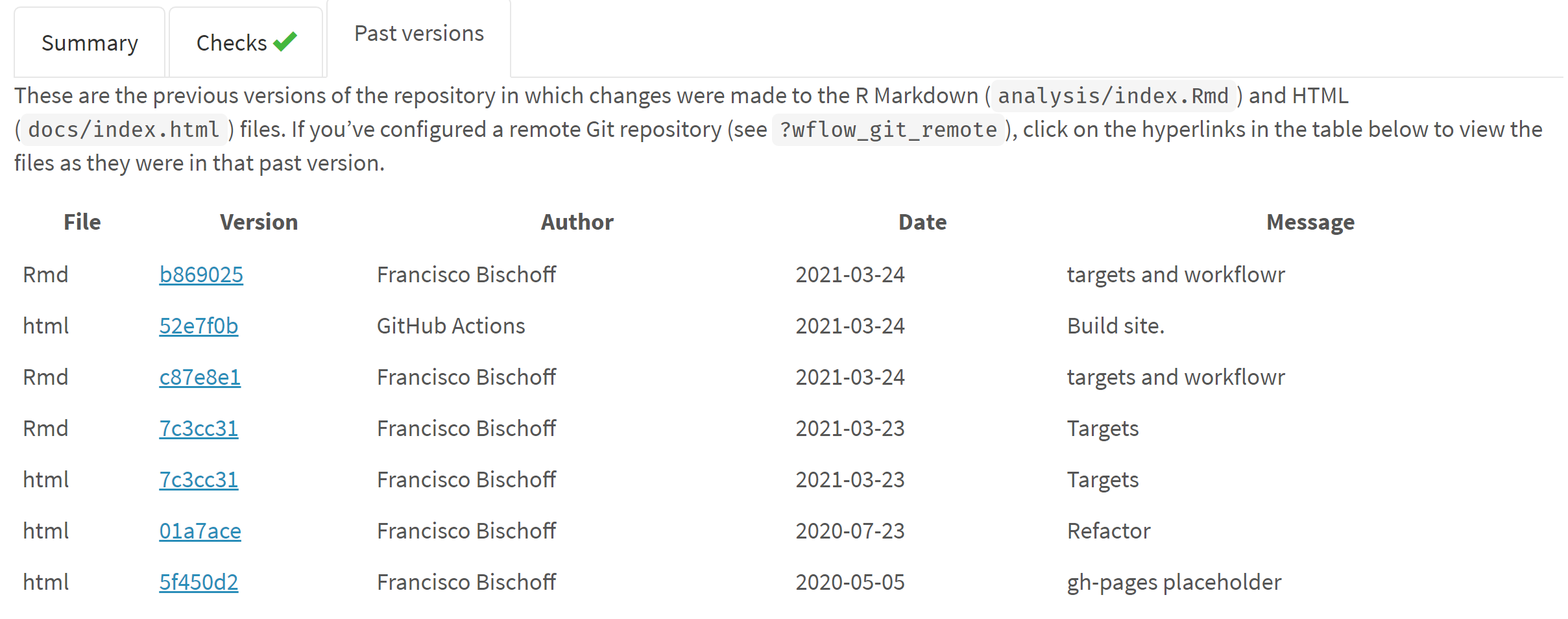
Figure 3.2: Fraction of the website generated by workflowr. On top we see that this version passed all checks, and in the middle we see a table referring to the previous versions of the report.
| Version | Author | Date |
|---|---|---|
| 1473a05 | Francisco Bischoff | 2021-07-15 |
3.1.3 Modeling and parameter tuning
The well-known package used for data science in R is the caret (short for Classification
And REgression Training)7. Nevertheless, the author of caret recognizes
several limitations of his (great) package and is now in charge of developing the tidymodels8 collection. For sure, there are other available frameworks and opinions9. Notwithstanding, this project will follow the tidymodels road. Three significant
arguments 1) constantly improving and constantly being re-checked for bugs; large community
contribution; 2) allows to plug in a custom modeling algorithm that, in this case, will be the one
needed for developing this work; 3) caret is not in active development.
3.1.4 Continuous integration
Meanwhile, the project pipeline has been set up on GitHub, Inc.10, leveraging Github Actions11 for the Continuous Integration lifecycle. The repository is available at10, and the resulting report is available at5. This thesis’s roadmap and tasks status are also publicly available on Zenhub12.
3.2 Developed software
3.2.1 Matrix Profile
Matrix Profile (MP)13 is a state-of-the-art14,15 time series analysis technique that, once computed, allows us to derive frameworks to all sorts of tasks, as motif discovery, anomaly detection, regime change detection, and others13.
Before MP, time series analysis relied on the distance matrix (DM), a matrix that stores all the distances between two time series (or itself, in the case of a Self-Join). This was very power-consuming, and several pruning and dimensionality reduction methods were researched16.
For brevity, let’s just understand that the MP and the companion Profile Index (PI) are two vectors that hold one floating-point value and one integer value, respectively, regarding the original time series: (1) the similarity distance between that point on time (let’s call these points “indexes”) and its first nearest-neighbor (1-NN), (2) The index where this 1-NN is located. The original paper has more detailed information13. It is computed using a rolling window, but instead of creating a whole DM, only the minimum values and the index of these minima are stored (in the MP and PI, respectively). We can have an idea of the relationship of both on Fig. 3.3.
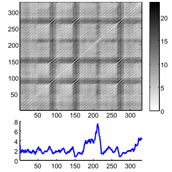
Figure 3.3: A distance matrix (top), and a matrix profile (bottom). The matrix profile stores only the minimum values of the distance matrix.
| Version | Author | Date |
|---|---|---|
| 0efd716 | Francisco Bischoff | 2022-02-02 |
This research has already yielded two R packages concerning the MP algorithms from UCR17. The
first package is called tsmp, and a paper has also been published in the R Journal18
(Journal Impact Factor™, 2020 of 3.984). The second package is called matrixprofiler and enhances
the first one, using low-level language to improve computational speed. The author has also joined
the Matrix Profile Foundation as a co-founder with contributors from Python and Go languages19,20.
This implementation in R is being used for computing the MP and MP-based algorithms of this thesis.
3.3 The data
The current dataset used is the CinC/Physionet Challenge 2015 public dataset, modified to include only the actual data and the header files in order to be read by the pipeline and is hosted by Zenodo21 under the same license as Physionet.
The dataset is composed of 750 patients with at least five minutes records. All signals have been resampled (using anti-alias filters) to 12 bit, 250 Hz, FIR band-pass (0.05 to 40Hz), and mains notch filters applied to remove noise. Pacemaker and other artifacts are still present on the ECG22. Furthermore, this dataset contains at least two ECG derivations and one or more variables like arterial blood pressure, photoplethysmograph readings, and respiration movements.
The events we seek to identify are the life-threatening arrhythmias as defined by Physionet in Table 3.1.
| Alarm | Definition |
|---|---|
| Asystole | No QRS for at least 4 seconds |
| Extreme Bradycardia | Heart rate lower than 40 bpm for 5 consecutive beats |
| Extreme Tachycardia | Heart rate higher than 140 bpm for 17 consecutive beats |
| Ventricular Tachycardia | 5 or more ventricular beats with heart rate higher than 100 bpm |
| Ventricular Flutter/Fibrillation | Fibrillatory, flutter, or oscillatory waveform for at least 4 seconds |
The fifth minute is precisely where the alarm has been triggered on the original recording set. To meet the ANSI/AAMI EC13 Cardiac Monitor Standards23, the onset of the event is within 10 seconds of the alarm (i.e., between 4:50 and 5:00 of the record). That doesn’t mean that there have been no other arrhythmias before.
For comparison, on Table 3.2 we collected the score of the five best participants of the challenge24–28.
| Score | Authors |
|---|---|
| 81.39 | Filip Plesinger, Petr Klimes, Josef Halamek, Pavel Jurak |
| 79.44 | Vignesh Kalidas |
| 79.02 | Paula Couto, Ruben Ramalho, Rui Rodrigues |
| 76.11 | Sibylle Fallet, Sasan Yazdani, Jean-Marc Vesin |
| 75.55 | Christoph Hoog Antink, Steffen Leonhardt |
The Equation used on this challenge to compute the score of the algorithms is in the Equation \(\eqref{score}\). This Equation is the accuracy formula, with the penalization of the false negatives. The reasoning pointed out by the authors22 is the clinical impact of existing an actual life-threatening event that was considered unimportant. Accuracy is known to be misleading when there is a high class imbalance29.
\[
Score = \frac{TP+TN}{TP+TN+FP+5*FN} \tag{1} \label{score}
\]
Assuming that this is a finite dataset, the pathologic cases (1) \(\lim_{TP \to \infty}\) (whenever there is an event, it is positive) or (2) \(\lim_{TN \to \infty}\) (whenever there is an event, it is false), cannot happen. This dataset has 292 True alarms and 458 False alarms. Experimentally, this equation yields:
- 0.24 if all guesses are on False class
- 0.28 if random guesses
- 0.39 if all guesses are on True class
- 0.45 if no false positives plus random on True class
- 0.69 if no false negatives plus random on False class
This small experiment (knowing the data in advance) shows that “a single line of code and a few minutes of effort”30 algorithm could achieve at most a score of 0.39 in this challenge (the last two lines, the algorithm must be very good on one class).
Nevertheless, this Equation will only be helpful to allow us to compare the results of this thesis with other algorithms.
3.4 Work structure
3.4.1 Project start
The project started with a literature survey on the databases Scopus, PubMed, Web of Science, and Google Scholar with the following query (the syntax was adapted for each database):
TITLE-ABS-KEY ( algorithm OR ‘point of care’ OR ‘signal processing’ OR ‘computer
assisted’ OR ‘support vector machine’ OR ‘decision support system’ OR ’neural
network’ OR ‘automatic interpretation’ OR ‘machine learning’) AND TITLE-ABS-KEY
( electrocardiography OR cardiography OR ‘electrocardiographic tracing’ OR ecg
OR electrocardiogram OR cardiogram ) AND TITLE-ABS-KEY ( ‘Intensive care unit’ OR
‘cardiologic care unit’ OR ‘intensive care center’ OR ‘cardiologic care center’ )
The inclusion and exclusion criteria were defined as in Table 3.3.
| Inclusion criteria | Exclusion criteria |
|---|---|
| ECG automatic interpretation | Manual interpretation |
| ECG anomaly detection | Publication older than ten years |
| ECG context change detection | Do not attempt to identify life-threatening arrhythmias, namely asystole, extreme bradycardia, extreme tachycardia, ventricular tachycardia, and ventricular flutter/fibrillation |
| Online Stream ECG analysis | No performance measurements reported |
| Specific diagnosis (like a flutter, hyperkalemia, etc.) |
The survey is being conducted with peer review; all articles on full-text phase were obtained and assessed for the extraction phase, except 5 articles that were not available. Due to external factors, the survey is currently stalled in the Data Extraction phase.
Fig. 3.4 shows the flow diagram of the resulting screening using PRISMA format.
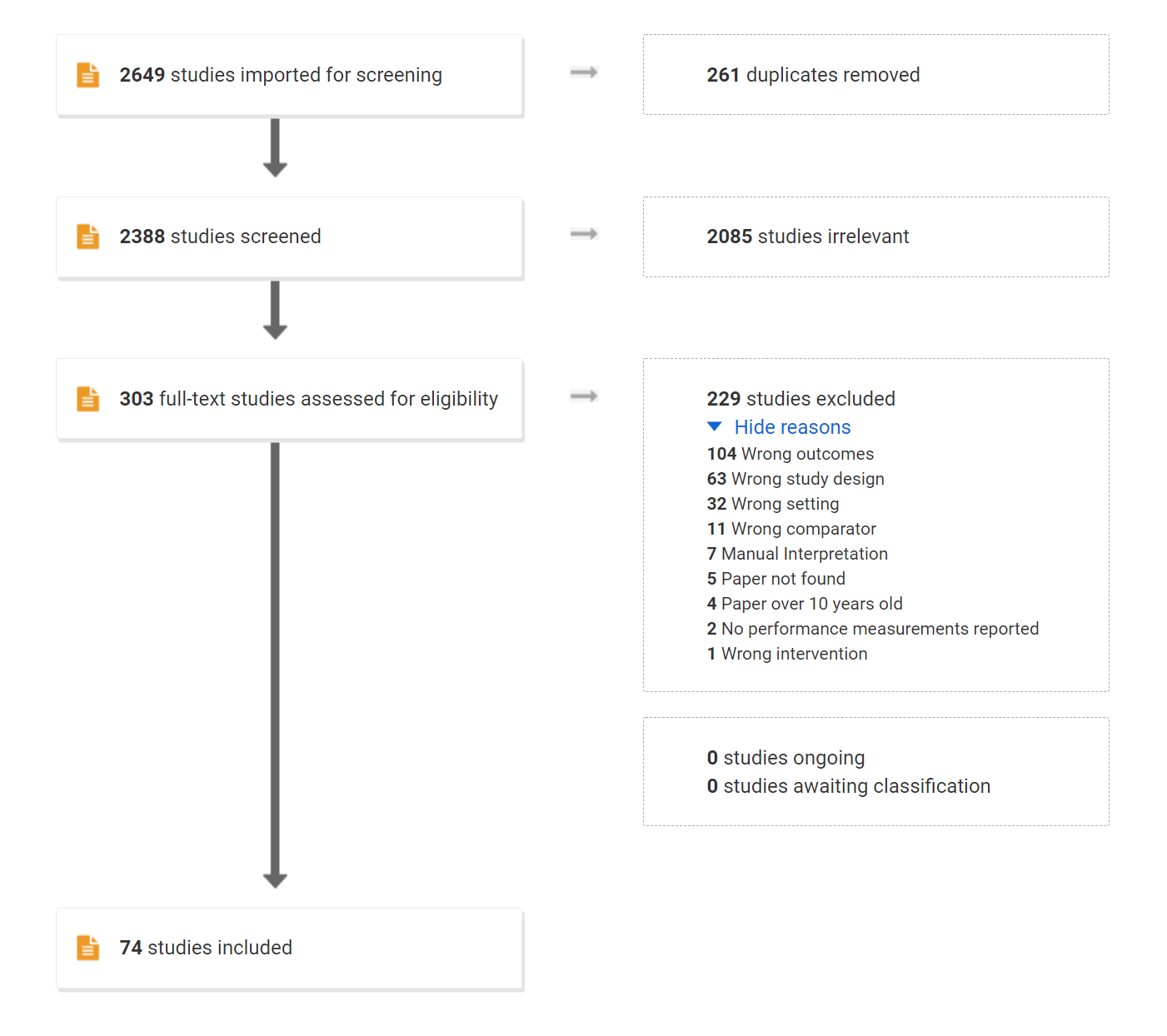
Figure 3.4: Flowchart of the literature survey.
| Version | Author | Date |
|---|---|---|
| 1473a05 | Francisco Bischoff | 2021-07-15 |
The peer review is being conducted by the author of this thesis and another colleague, Dr. Andrew Van Benschoten, from the Matrix Profile Foundation19.
Table. 3.4 shows the Inter-rater Reliability (IRR) of the screening phases, using Cohen’s \(\kappa\) statistic. The bottom line shows the estimated accuracy after correcting possible confounders31.
|
Title-Abstract (2388 articles) |
Full-Review (303 articles) |
|||||
|---|---|---|---|---|---|---|
| Reviewer #2 | Reviewer #2 | |||||
| Include | Exclude | Include | Exclude | |||
| Reviewer #1 | Include | 185 | 381 | 63 | 58 | |
| Exclude | 129 | 1693 | 13 | 169 | ||
| Cohen’s omnibus \(\kappa\) | 0.30 | 0.48 | ||||
| Maximum possible \(\kappa\) | 0.66 | 0.67 | ||||
| Std Err for \(\kappa\) | 0.02 | 0.05 | ||||
| Observed Agreement | 79% | 77% | ||||
| Random Agreement | 69% | 55% | ||||
| Agreement corrected with KappaAcc | 82% | 85% | ||||
The purpose of using Cohen’s \(\kappa\) in such a review is to allow us to gauge the agreement of both reviewers on the task of selecting the articles according to the goal of the survey. The most naive way to verify this would be simply to measure the overall agreement (the number of articles included and excluded by both, divided by the total number of articles). Nevertheless, this would not take into account the agreement we could expect purely by chance.
However, the \(\kappa\) statistic must be assessed carefully. This topic is beyond the scope of this work therefore it will be explained briefly.
While it is widely used, the \(\kappa\) statistic is well criticized. The direct interpretation of its value depends on several assumptions that are often violated. (1) It is assumed that both reviewers have the same level of experience; (2) The “codes” (include, exclude) are identified with same accuracy; (3) The “codes” prevalences are the same; (4) There is no reviewer bias towards one of the choices32,33.
In addition, the number of “codes” affects the relation between the value of \(\kappa\) and the actual agreement between the reviewers. For example, given equiprobable “codes” and reviewers who are 85% accurate, the value of \(\kappa\) are 0.49, 0.60, 0.66, and 0.69 when number of codes is 2, 3, 5, and 10, respectively33,34.
To take into account these limitations, the agreement between reviewers was calculated using the KappaAcc31 from Professor Emeritus Roger Bakeman, Georgia State University, which computes the estimated accuracy of simulated reviewers.
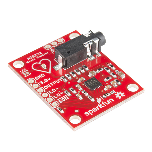
3.4.2 RAW data
To better understand the data acquisition, it has been acquired a Single Lead Heart Rate Monitor breakout from Sparkfun™35 using the AD823236 microchip from Analog Devices Inc., compatible with Arduino®37, for an in-house experiment (Fig. 3.5).
| Version | Author | Date |
|---|---|---|
| 1473a05 | Francisco Bischoff | 2021-07-15 |
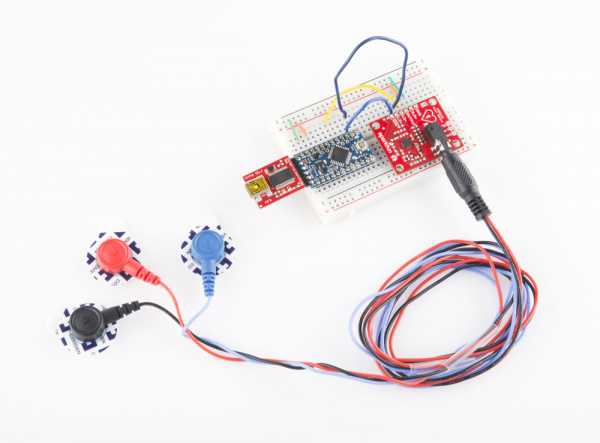
Figure 3.5: Single Lead Heart Rate Monitor.
| Version | Author | Date |
|---|---|---|
| 1473a05 | Francisco Bischoff | 2021-07-15 |
The output gives us a RAW signal, as shown in Fig. 3.6.
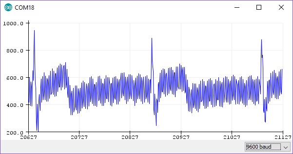
Figure 3.6: RAW output from Arduino at ~300hz.
| Version | Author | Date |
|---|---|---|
| 1473a05 | Francisco Bischoff | 2021-07-15 |
After applying the same settings as the Physionet database (collecting the data at 500hz, resample to 250hz, pass-filter, and notch filter), the signal is much better, as shown in Fig. 3.7.
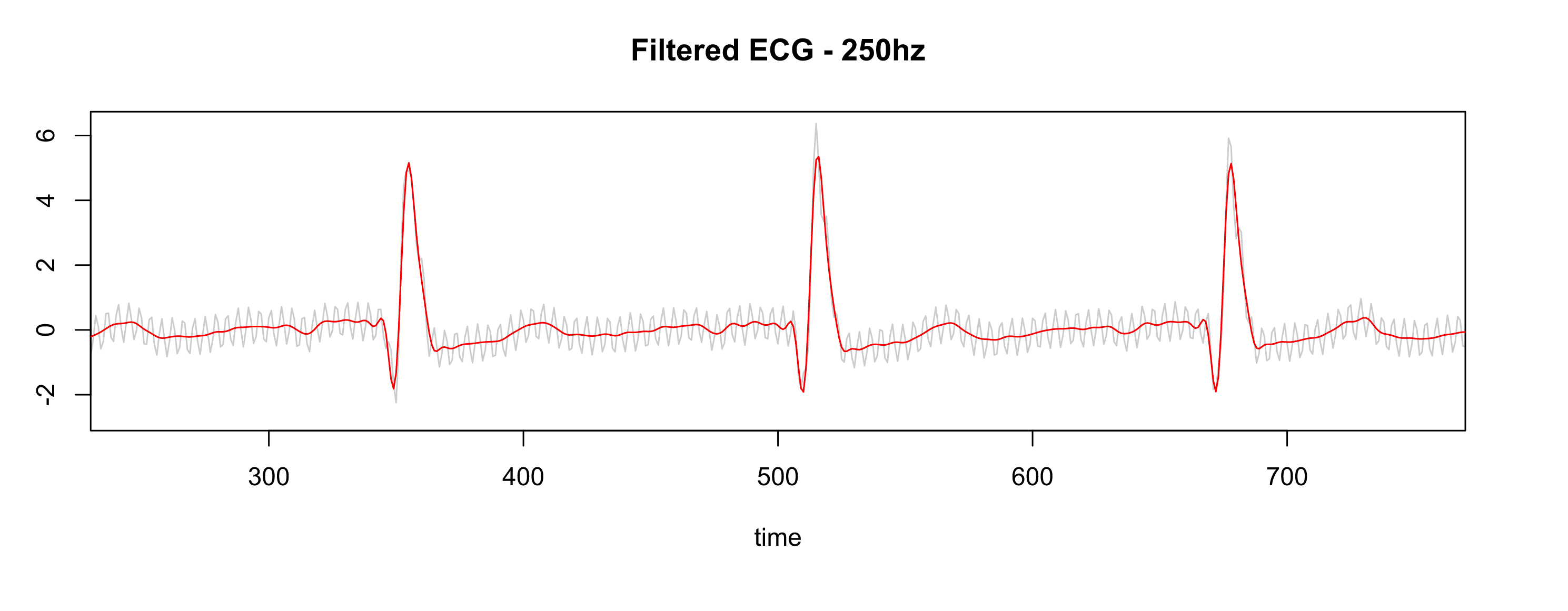
Figure 3.7: Gray is RAW, Red is filtered.
| Version | Author | Date |
|---|---|---|
| 1473a05 | Francisco Bischoff | 2021-07-15 |
3.4.3 Preparing the data
Usually, data obtained by sensors needs to be “cleaned” for proper evaluation. That is different from the initial filtering process where the purpose is to enhance the signal. Here we are dealing with artifacts, disconnected cables, wandering baselines and others.
Several SQIs (Signal Quality Indexes) are used in the literature38, some trivial measures as kurtosis, skewness, median local noise level, other more complex as pcaSQI (the ratio of the sum of the five largest eigenvalues associated with the principal components over the sum of all eigenvalues obtained by principal component analysis applied to the time aligned ECG segments in the window). An assessment of several different methods to estimate electrocardiogram signal quality can was performed by Del Rio, et al39.
By experimentation (yet to be validated), a simple formula gives us the “complexity” of the signal and correlates well with the noisy data is shown in Equation \(\eqref{complex}\)40.
\[
\sqrt{\sum_{i=1}^w((x_{i+1}-x_i)^2)}, \quad \text{where}\; w \; \text{is the window size} \tag{2} \label{complex}
\]
Fig. 3.8 shows some SQIs and their relation with the data.
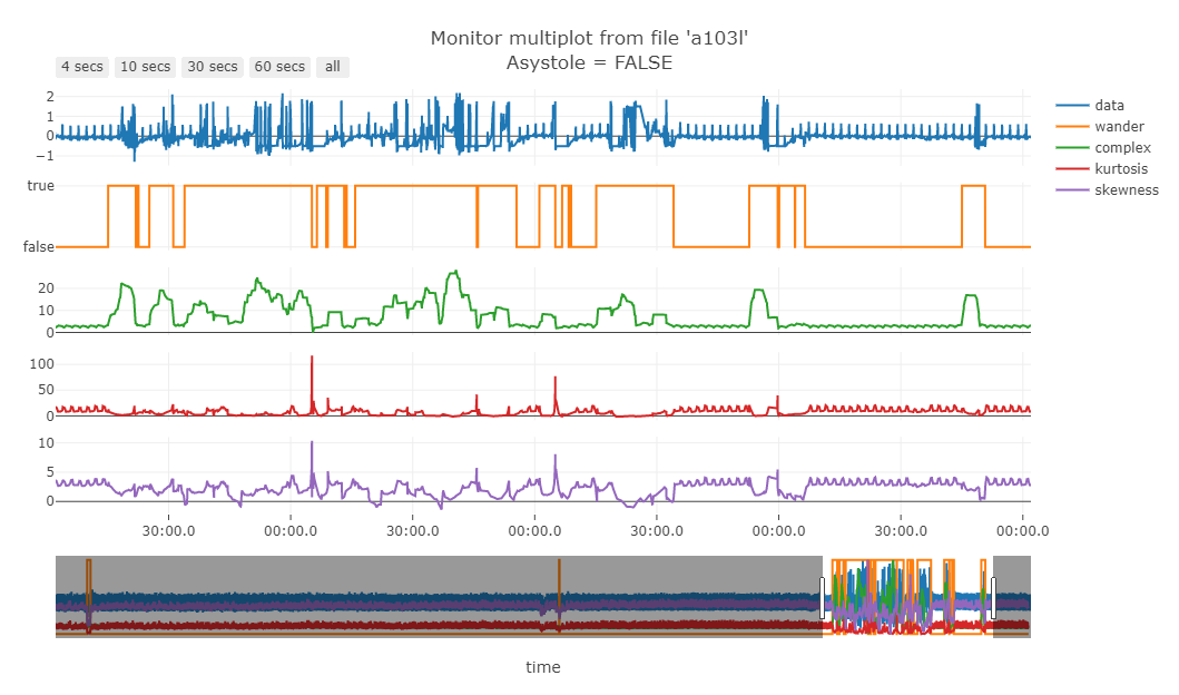
Figure 3.8: Green line is the “complexity” of the signal.
| Version | Author | Date |
|---|---|---|
| 1473a05 | Francisco Bischoff | 2021-07-15 |
Fig. 3.9 shows that noisy data (probably patient muscle movements) are marked with a blue point and thus are ignored by the algorithm.

Figure 3.9: Noisy data marked by the “complexity” filter.
Although this step of “cleaning” the data is often used, this step will also be tested if it is really necessary, and the performance with and without “cleaning” will be reported.
3.4.4 Detecting regime changes
The regime change approach will be using the Arc Counts concept, used on the FLUSS (Fast Low-cost Unipotent Semantic Segmentation) algorithm, as explained by Gharghabi, et al.,41.
The FLUSS (and FLOSS, the online version) algorithm is built on top of the Matrix Profile (MP)13, described on section 3.2.1. Recalling that the MP and the companion Profile Index (PI) are two vectors holding information about the 1-NN. One can imagine several “arcs” starting from one “index” to another. This algorithm is based on the assumption that between two regimes, the most similar shape (its nearest neighbor) is located on “the same side”, so the number of “arcs” decreases when there is a change in the regime and increases again. As show on Fig. 3.10. This drop on the Arc Counts is a signal that a change in the shape of the signal has happened.

Figure 3.10: FLUSS algorithm, using arc counts.
| Version | Author | Date |
|---|---|---|
| 0efd716 | Francisco Bischoff | 2022-02-02 |
The choice of the FLOSS algorithm (the online version of FLUSS) is founded on the following arguments:
- Domain Agnosticism: the algorithm makes no assumptions about the data as opposed to most available algorithms to date.
- Streaming: the algorithm can provide real-time information.
- Real-World Data Suitability: the objective is not to explain all the data. Therefore, areas marked as “don’t know” areas are acceptable.
- FLOSS is not: a change point detection algorithm42. The interest here is changes in the shapes of a sequence of measurements.
Other algorithms we can cite are based on Hidden Markov Models (HMM) that require at least two parameters to be set by domain experts: cardinality and dimensionality reduction. The most attractive alternative could be the Autoplait43, which is also domain agnostic and parameter-free. It segments the time series using Minimum Description Length (MDL) and recursively tests if the region is best modeled by one or two HMM. However, Autoplait is designed for batch operation, not streaming, and also requires discrete data. FLOSS was demonstrated to be superior in several datasets in its original paper. In addition, FLOSS is robust to several changes in data like downsampling, bit depth reduction, baseline wandering, noise, smoothing, and even deleting 3% of the data and filling with simple interpolation. Finally, the most important, the algorithm is light and suitable for low-power devices.
In the MP domain, it is worth also mentioning another possible algorithm: the Time Series Snippets44, based on MPdist45. The MPdist measures the distance between two sequences, considering how many similar sub-sequences they share, no matter the matching order. It proved to be a useful measure (not a metric) for meaningfully clustering similar sequences. Time Series Snippets exploits MPdist properties to summarize a dataset extracting the \(k\) sequences representing most of the data. The final result seems to be an alternative for detecting regime changes, but it is not. The purpose of this algorithm is to find which pattern(s) explains most of the dataset. Also, it is not suitable for streaming data. Lastly, MPdist is quite expensive compared to the trivial Euclidean distance.
The regime change detection will be evaluated following the criteria explained in section 3.5.
3.4.5 Classification of the new regime
The next step towards the objective of this work is to verify if the new regime detected by the previous step is indeed a life-threatening pattern that we should trigger the alarm.
First, let’s dismiss some apparent solutions: (1) Clustering. It is well understood that we cannot cluster time series subsequences meaningfully with any distance measure or with any algorithm46. The main argument is that in a meaningful algorithm, the output depends on the input, and this has been proven to not happen in time series subsequence clustering46. (2) Anomaly detection. In this work, we are not looking for surprises but for patterns that are known to be life-threatening. (3) Forecasting. We may be tempted to make predictions, but this clearly is not the idea here.
The method of choice is classification. The simplest algorithm could be a TRUE/FALSE binary
classification. Nevertheless, the five life-threatening patterns have well-defined characteristics
that may seem more plausible to classify the new regime using some kind of ensemble of binary
classifiers or a “six-class” classifier (the sixth class being the FALSE class).
Since the model doesn’t know which life-threatening pattern will be present in the regime (or if it
will be a FALSE case), the model will need to check for all five TRUE cases, and if none of
these cases are identified, it will classify the regime as FALSE.
To avoid exceeding processor capacity, an initial set of shapelets47 can be
sufficient to build the TRUE/FALSE classifier. And to build such a set of shapelets, leveraging
on the MP, we will use the Contrast Profile48.
The Contrast Profile (CP) looks for patterns that are at the same time very similar to its neighbors in class A while is very different from the nearest neighbor from class B. In other words, this means that such a pattern represents well class A and may be taken as a “signature” of that class.
In this case, we need to compute two MP, one self-join MP using the positive class \(MP^{(++)}\) (the class that has the signature we want to find) and one AB-join MP using the positive and negative classes \(MP^{(+-)}\). Then we subtract the first \(MP^{(++)}\) from the last \(MP^{(+-)}\), resulting in the \(CP\). The high values on \(CP\) are the locations for the signature candidates we look for (the author of CP calls these segments Plato’s).
Due to the nature of this approach, the MP’s (containing values in Euclidean Distance) are truncated for values above \(\sqrt{2w}\), where \(w\) is the window size. This is because values above this threshold are negatively correlated in the Pearson Correlation space. Finally, we normalize the values by \(\sqrt{2w}\). The formula \(\eqref{contrast}\) synthesizes this computation.
\[
CP_w = \frac{MP_{w}^{(+-)} - MP_{w}^{(++)}}{\sqrt{2w}} \quad \text{where}\; w \; \text{is the window size} \tag{3} \label{contrast}
\]
For a more complete understanding of the process, Fig. 3.11 shows a practical example from the original article48.

Figure 3.11: Top to bottom: two weakly-labeled snippets of a larger time series. T(-) contains only normal beats. T(+) also contains PVC (premature ventricular contractions). Next, two Matrix Profiles with window size 91; AB-join is in red and self-join in blue. Bottom, the Contrast Profile showing the highest location.
| Version | Author | Date |
|---|---|---|
| 0efd716 | Francisco Bischoff | 2022-02-02 |
After extracting candidates for each class signature, a classification algorithm will be fitted and evaluated using the criteria explained on section 3.5.
3.4.6 Summary of the methodology
To summarize the steps taken on this thesis to accomplish the main objective, Figs. 3.13, 3.14 and 3.15 show the overview of the processes involved.
First, let us introduce the concept of Nested Resampling49. It is known that when increasing model complexity, overfitting on the training set becomes more likely to happen50. This is an issue that this work has to countermeasure as many steps require parameter tuning, even for almost parameter-free algorithms, like the MP.
The rule that must be followed is simple: do not evaluate a model on the same resampling split used to perform its own parameter tuning. Using simple cross-validation, the information about the test set “leaks” into the evaluation, leading to overfitting/overtuning, and gives us an optimistic biased estimate of the performance. Bernd Bischl, 201249 describes more deeply these factors and also provides us with a countermeasure for that: (1) from preprocessing the data to model selection use the training set; (2) the test set should be touched once, on the evaluation step; (3) repeat. This guarantees that a “new” separated data is only used after the model is trained/tuned.
Fig. 3.12 shows us this principle. The steps (1) and (2) described above are part of the Outer resampling, which in each loop splits the data into two sets: the training set and the test set. The training set is then used in the Inner resampling where, for example, the usual cross-validation may be used (creating an Analysis set and an Assessment set to avoid terminology conflict), and the best model/parameters are selected. Then, this best model is evaluated against the unseen test set created for this resampling.
The resulting (aggregated) performance of all outer samples gives us a more honest estimative of the expected performance on new data.

Figure 3.12: Nested resampling. The full dataset is resampled several times (outer resampling), so each branch has its own Test set (yellow). On each branch, the Training set is used as if it were a full dataset, being resampled again (inner resampling); here, the Assessment set (blue) is used to test the learning model and tune parameters. The best model is finally evaluated on its own Test set.
| Version | Author | Date |
|---|---|---|
| 0efd716 | Francisco Bischoff | 2022-02-02 |
After the understanding of the Nested Resampling49, the following flowcharts can be better interpreted. Fig. 3.13 starts with the “Full Dataset” that contains all time series from the dataset described in section 3.3. Each time series represents one file from the database and represents one patient.
The regime change detection will use subsampling (bootstrapping can lead to substantial bias toward more complex models) in the Outer resampling and cross-validation in the Inner resampling. How the evaluation will be performed and why the use of cross-validation will be explained in section 3.5.

Figure 3.13: Pipeline for regime change detection. The full dataset (containing several patients) is divided into a Training set and a Test set. The Training set is then resampled in an Analysis set and an Assessment set. The former is used for training/parameter tuning and the latter for assessing the result. The best parameters are then used for evaluation on the Test set. This may be repeated several times.
| Version | Author | Date |
|---|---|---|
| 0efd716 | Francisco Bischoff | 2022-02-02 |
Fig. 3.14 shows the processes for training the classification model. First, the
last ten seconds of each time series will be identified (the event occurs in this segment). Then the
dataset will be grouped by class (type of event) and TRUE/FALSE (alarm), so the Outer/Inner
resampling will produce a Training/Analysis set and Test/Assessment set with similar frequency to
the full dataset.
The next step will be to extract shapelet candidates using the Contrast Profile and train the classifier.
This pipeline will use subsampling (for the same reason above) in the Outer resampling and cross-validation in the Inner resampling. How the evaluation will be performed and why the use of cross-validation will be explained in section 3.5.

Figure 3.14: Pipeline for alarm classification. The full dataset (containing several patients) is grouped by class and by TRUE/FALSE alarm. This grouping allows resampling to keep a similar frequency of classes and TRUE/FALSE of the full dataset. Then the full dataset is divided on a Training set and a Test set. The Training set is then resampled in an Analysis set and an Assessment set. The former is used for extracting shapelets, training the model and parameter tuning; the latter for assessing the performance of the model. Finally, the best model is evaluated on the Test set. This may be repeated several times.
| Version | Author | Date |
|---|---|---|
| 0efd716 | Francisco Bischoff | 2022-02-02 |
Finally, Fig. 3.15 shows how the final model will be used on the field. In a streaming scenario, the data will be collected and processed in real-time to maintain an up to date Matrix Profile. The FLOSS algorithm will be looking for a regime change. When a regime change is detected, a sample of this new regime will be presented to the trained classifier that will evaluate if this new regime is a life-threatening condition or not.

Figure 3.15: Pipeline of the final process. The streaming data, coming from one patient, is processed to create its Matrix Profile. Then, the FLOSS algorithm is computed for detecting a regime change. When a new regime is detected, a sample of this new regime is analysed by the model and a decision is made. If the new regime is life-threatening, the alarm will be fired.
| Version | Author | Date |
|---|---|---|
| 0efd716 | Francisco Bischoff | 2022-02-02 |
3.5 Evaluation of the algorithms
The subsampling method used on both algorithms, regime change, and classification, will be the Cross-Validation, as the learning task will be in batches.
Other options dismissed49:
Leave-One-Out Cross-Validation: has better properties for regression than for classification. It has a high variance as an estimator of the mean loss. It also is asymptotically inconsistent and tends to select too complex models. It is demonstrated empirically that 10-fold CV is often superior.
Bootstrapping: while it has low variance, it may be optimistic-biased on more complex models. Also, its resampling method with replacement can leak information into the assessment set.
Subsampling: is like bootstrapping, but without replacement. The only argument for not choosing it is that we make sure all the data is used for analysis and assessment with Cross-Validation.
3.5.1 Regime change
A detailed discussion about the evaluation process of segmentation algorithms is made by the FLUSS/FLOSS author41. Previous researches have used precision/recall or derived measures for performance. The main issue is how to assume that the algorithm was correct? Is this a miss if the ground truth says the change occurred at location 10,000, and the algorithm detects a change at location 10,001?
As pointed out by the author, several independent researchers have suggested a temporal tolerance, that solves one issue but has a hard time penalizing any tiny miss beyond this tolerance.
The second issue is an over-penalization of an algorithm in which most of the detections are good, but just one (or a few) is poor.
The author proposes the solution depicted in Fig. 3.16. It gives 0 as the best score and 1 as the worst. The function sums the distances between the ground truth locations and the locations suggested by the algorithm. The sum is then divided by the length of the time series to normalize the range to [0, 1].
The goal is to minimize this score.

Figure 3.16: Regime change evaluation. The top line illustrates the ground truth, and the bottom line the locations reported by the algorithm. Note that multiple proposed locations can be mapped to a single ground truth point.
| Version | Author | Date |
|---|---|---|
| 0efd716 | Francisco Bischoff | 2022-02-02 |
3.5.2 Classification
As described in section 3.4.5, the model for classification will use a set of shapelets
to identify if we have a TRUE (life-threatening) regime or a FALSE (non-life-threatening) regime.
Although the implementation of the final process will be using streaming data, the classification algorithm will work in batches because it will not be applied on every single data point but on samples that are extracted when a regime change is detected. During the training phase, the data is also analyzed in batches.
One important factor we must consider is that, in real-world, the majority of regime changes will be
FALSE (i.e., not life-threatening). Thus, a performance measure that is robust to class imbalance
is needed if we want to assess the model after it was trained on the field.
It is well known that the Accuracy measure is not reliable for unbalanced data29,51 as it returns optimistic results for a classifier on the majority class. A description of common measures used on classification is available29,52. Here we will focus on three candidate measures that can be used: F-score (well discussed on52), Matthew’s Correlation Coefficient (MCC)53 and \(\kappa_m\) statistic54.
The F-score (let’s abbreviate to F1 as this is the more common setting) is widely used on
information retrieval, where the classes are usually classified as “relevant” and “irrelevant”,
and combines the recall (also known as sensitivity) and the precision (the positive predicted
value). Recall assess how well the algorithm retrieves relevant examples among the (usually few)
relevant items in the dataset. In contrast, precision assesses the proportion of indeed relevant
items which are contained in the retrieved examples. It ranges from [0, 1]. It completely ignores
the irrelevant items that were not retrieved (usually, this set contains many items). In
classification tasks, its main weakness is not evaluating the True Negatives. If the proportion of a
random classifier gets towards the TRUE class (increasing the False Positives significantly), this
score actually gets better, thus not suitable to our case. The F1 score is defined on Equation
\(\eqref{score}\).
\[ F_1 score = \frac{2 \cdot TP}{2 \cdot TP + FP + FN} = 2 \cdot \frac{precision \cdot recall}{precision + recall} \tag{4} \label{fscore} \]
The MCC is a good alternative to the F1 when we do care about the True negatives (both were considered to “provide more realistic estimates of real-world model performance”55). It is a method to compute the Pearson product-moment correlation coefficient56 between the actual and predicted values. It ranges from [-1, 1]. The MCC is the only binary classification rate that only gives a high score if the binary classifier correctly classified the majority of the positive and negative instances52. One may argue that Cohen’s \(\kappa\) has the same behavior. Still, there are two main differences (1) MCC is undefined in the case of a majority voter. At the same time, Cohen’s \(\kappa\) doesn’t discriminate this case from the random classifier (\(\kappa\) is zero for both cases). (2) It is proven that in a special case when the classifier is increasing the False Negatives, Cohen’s \(\kappa\) doesn’t get worse as expected, MCC doesn’t have this issue56. MCC is defined on equation \(\eqref{mccval}\).
\[ MCC = \frac{TP \cdot TN - FP \cdot FN}{\sqrt{(TP + FP) \cdot (TP + FN) \cdot (TN + FP) \cdot (TN + FN)}} \tag{5} \label{mccval} \]
The \(\kappa_m\) statistic54 is a measure that considers not the random classifier but the majority voter (a classifier that only votes on the larger class). It was introduced by Bifet et al.54 for being used in online settings, where the class balance may change over time. It is defined on Equation \(\eqref{kappam}\), where \(p_0\) is the observed accuracy, and \(p_m\) is the accuracy of the majority voter. Theoretically, the score ranges from (\(-\infty\), 1]. Still, in practice, you see negative numbers if the classifier performs worse than the majority voter and positive numbers if performing better than the majority number until the maximum of 1 when the classifier is optimal.
\[ \kappa_m = \frac{p_0 - p_m}{1 - p_m} \tag{6} \label{kappam} \]
In the inner resampling (model training/tuning), the classification will be binary, and in our case, we know that the data is slightly unbalanced (60% false alarms). For this step, the metric for model selection will be the MCC. Nevertheless, during the optimization process, the algorithm will seek to minimize the False Negative Rate (\(FNR = \frac{FN}{TP+FN}\)), and between ties, the smaller FNR wins.
In the outer resampling, the MCC and \(\kappa_m\) of all winning models will aggregate and report using the median and interquartile range.
For different classifiers, we will use Wilcoxon’s signed-rank test for comparing their performances. This method is known to have low Type I and Type II errors in this kind of comparison54.
3.5.3 Full model (streaming setting)
For the final assessment, the best and the average model of the previous pipelines will be assembled and tested using the whole original dataset.
The algorithm will be tested in each of the five life-threatening events split individually in order to evaluate its strengths and weakness.
For more transparency, the whole confusion matrix will be reported, as well as the MCC, \(\kappa_m\), and the FLOSS evaluation.
4 Current results
4.1 Regime change detection
As we have seen previously, the FLOSS algorithm is built on top of the Matrix Profile (MP). Thus, we have proposed several parameters that may or not impact the FLOSS prediction performance.
The variables for building the MP are:
mp_threshold: the minimum similarity value to be considered for 1-NN.time_constraint: the maximum distance to look for the nearest neighbor.window_size: the default parameter always used to build an MP.
Later, the FLOSS algorithm also has a parameter that needs tuning to optimize the prediction:
regime_threshold: the threshold below which a regime change is considered.regime_landmark: the point in time where the regime threshold is applied.
Using the tidymodels framework, we performed a basic grid search on all these parameters.
Fig. 4.1 shows the workflow using Nested resamplig as described on section 3.4.6. Fig. 4.2 shows an example of the regime change detection pipeline. The graph on top shows the ECG streaming; the blue line marks the ten seconds before the original alarm was fired; the red line marks the time constraint used on the example; the dark red line marks the limit for taking a decision in this case of Asystole; The blue horizontal line represents the size of the sliding window. The graph on the middle shows the Arc counts as seen by the algorithm (with the corrected distribution); the red line marks the current minimum value and its index; the blue horizontal line shows the minimum value seen until then. The graph on the bottom shows the computed Arc counts (raw) and the red line is the theoretical distribution used for correction.
Figure 4.1: FLOSS pipeline.
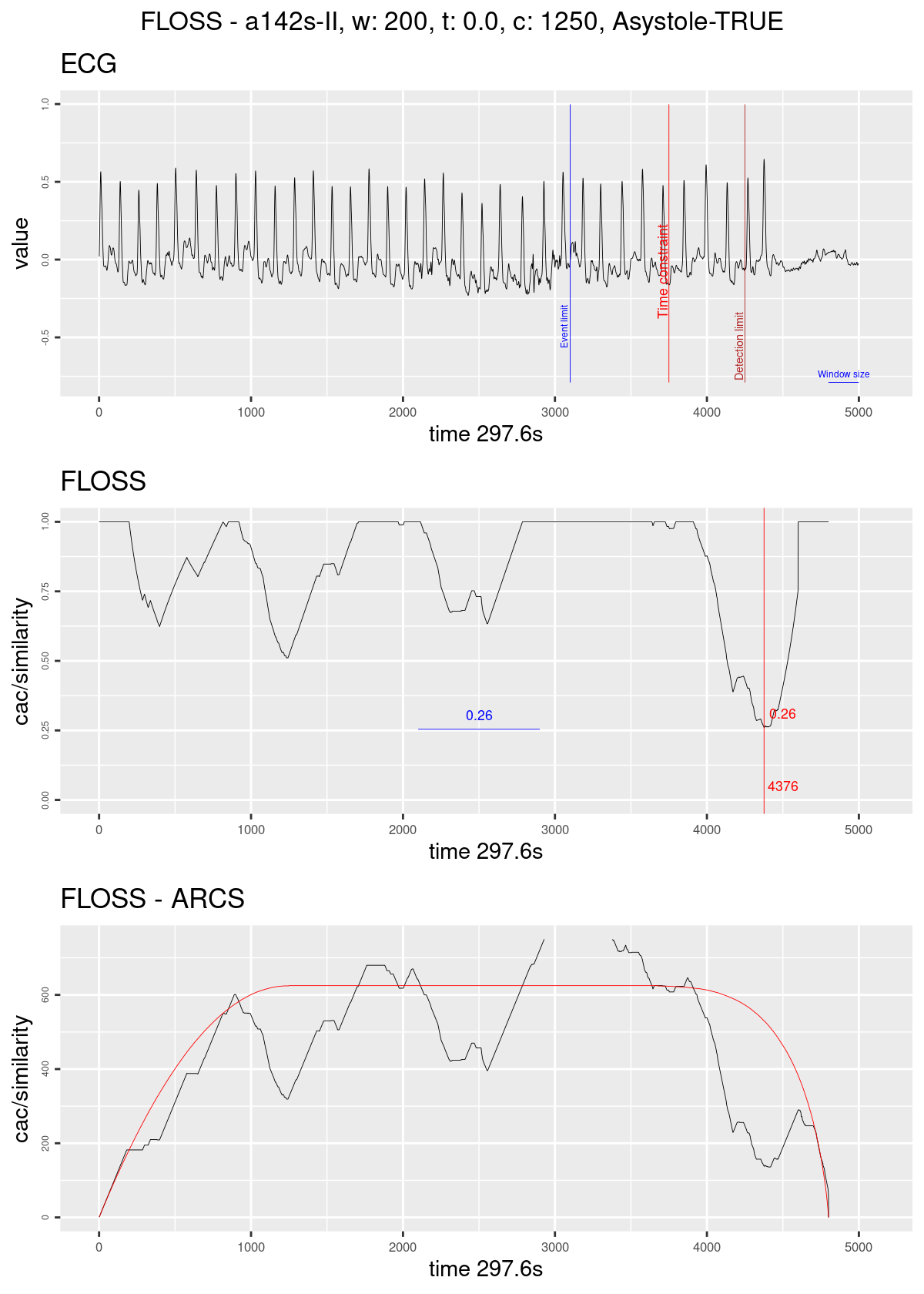
Figure 4.2: Regime change detection example. The graph on top shows the ECG streaming; the blue line marks the ten seconds before the original alarm was fired; the red line marks the time constraint of 1250; the dark red line marks the limit for taking a decision in this case of Asystole the blue horizontal line represents the size of the sliding window. The graph on the middle shows the Arc counts as seen by the algorithm (with the corrected distribution); the red line marks the current minimum value and its index; the blue horizontal line shows the minimum value seen until then. The graph on the bottom shows the computed Arc counts (raw), and the red line is the theoretical distribution used for correction.
| Version | Author | Date |
|---|---|---|
| 0efd716 | Francisco Bischoff | 2022-02-02 |
The dataset used for working with the Regime Change algorithm was the “Paroxysmal Atrial Fibrillation Events Detection from Dynamic ECG Recordings: The 4th China Physiological Signal Challenge 2021” hosted by Zenodo57 under the same license as Physionet.
The selected records were those that contain paroxysmal atrial fibrillation events, a total of 229 records. The records were split in a proportion of 3/4 for the training set (inner resampling) and 1/4 for the test set (outer resampling). The inner resampling was performed using a 5-fold cross-validation, which accounts for 137 records for fitting the models and 92 records for assessing them in the inner resampling.
The following parameters were used:
- The MP parameters were explored using the following values:
mp_threshold: 0.0 to 0.9, by 0.1 steps;time_constraint: 0, 800 and 1500;window_size: 25 to 350, by 25 steps;
- The FLOSS parameters were explored using the following values:
regime_threshold: 0.05 to 0.90, by 0.05 steps;regime_landmark: 1 to 10, by 0.5 steps.
4.1.1 Parameters analysis
The above process was an example of parameter tuning seeking the best model for a given set of parameters. It used a nested cross-validation procedure that aims to find the best combination of parameters and avoid overfitting.
While this process is powerful and robust, it does not show us the importance of each parameter. At least one parameter has been introduced by reasoning about the problem (mp_threshold), but how important it (and other parameters) is for predicting regime changes?
For example, the process above took 4 days, 20 hours, and 15 minutes to complete the grid search using an Intel(R) Xeon(R) Silver 4210R @ 2.40 GHz server. Notice that about 133 different combinations of parameters were tested on computing the MP (not FLOSS, the regime_threshold), 5 folds, 2 times each. That sums up about 35.2 x 10⁹ all-pairs Euclidean distances computed on less than 5 days (on CPU, not GPU). Not bad.
Another side note on the above process, it is not a “release” environment, so we must consider lots of overhead in computation and memory usage that must be taken into account during these five days of grid search. Thus, much time can be saved if we know what parameters are essential for the problem.
In order to check the effect of the parameters on the model, we need to compute the importance of each parameter.
Wei et al. published a comprehensive review on variable importance analysis58.
Our case is not a typical case of variable importance analysis, where a set of features are tested against an outcome. Instead, we have to proxy our analysis by using as outcome the FLOSS performance score and as features (or predictors) the tuning parameters that lead to that score.
That is accomplished by fitting a model using the tuning parameters to predict the FLOSS score and then applying the techniques to compute the importance of each parameter.
For this matter, a Bayesian Additive Regression Trees (BART) model was chosen after an experimental trial with a set of regression models (including glmnet, gbm, mlp) and for its inherent characteristics, which allows being used for model-free variable selection59. The best BART model was selected using 10-fold cross-validation repeated 3 times, having great predictive power with an RMSE around 0.2 and an R2 around 0.99. With this fitted model, we could evaluate each parameter’s importance.
4.1.2 Interactions
Before starting the parameter importance analysis, we need to consider the parameter interactions since this is usually the weak spot of the analysis techniques.
The first BART model was fitted using the following parameters:
\[ \begin{aligned} E( score ) &= \alpha + time\_constraint\\ &\quad + mp\_threshold + window\_size\\ &\quad + regime\_threshold + regime\_landmark \end{aligned} \tag{7} \label{eq-first} \]
After checking the interactions, this is the refitted model:
\[ \begin{aligned} E( score ) &= \alpha + time\_constraint\\ &\quad + mp\_threshold + window\_size\\ &\quad + regime\_threshold + regime\_landmark\\ &\quad + \left(regime\_threshold \times regime\_landmark\right)\\ &\quad + \left(mp\_threshold \times regime\_landmark\right)\\ &\quad + \left(mp\_threshold \times window\_size\right) \end{aligned} \tag{8} \label{eq-fitted} \]
Fig. 4.3 shows the variable interaction strength between pairs of variables. That allows us to verify if there are any significant interactions between the variables. Using the information from the first model fit, equation \(\eqref{eq-first}\), we see that regime_threshold interacts strongly with regime_landmark. This interaction was already expected, and we see that even after refitting the model, equation \(\eqref{eq-fitted}\), this interaction is still strong.
This is not a problem per se but a signal we must be aware of when exploring the parameters.
![Variable interactions strength using feature importance ranking measure (FIRM) approach [@Greenwell2018]. A) Shows strong interaction between `regime_threshold` and `regime_landmark`, `mp_threshold` and `window_size`, `mp_threshold` and `regime_landmark`. B) Refitting the model with these interactions taken into account, the strength is substantially reduced, except for the first, showing that indeed there is a strong correlation between those variables.](figure/report.Rmd/interaction-1.svg)
Figure 4.3: Variable interactions strength using feature importance ranking measure (FIRM) approach60. A) Shows strong interaction between regime_threshold and regime_landmark, mp_threshold and window_size, mp_threshold and regime_landmark. B) Refitting the model with these interactions taken into account, the strength is substantially reduced, except for the first, showing that indeed there is a strong correlation between those variables.
| Version | Author | Date |
|---|---|---|
| 4887954 | Francisco Bischoff | 2023-08-13 |
4.1.3 Importance
After evaluating the interactions, we then can perform the analysis of the variable importance. The goal is to understand how the FLOSS score behaves when we change the parameters.
Here is a brief overview of the different techniques:
4.1.3.1 Feature Importance Ranking Measure (FIRM)
The FIRM is a variance-based method. This implementation uses the ICE curves to quantify each feature effect which is more robust than partial dependance plots (PDP)61.
It is also helpful to inspect the ICE curves to uncover some heterogeneous relationships with the outcome62.
Advantages:
- Has a causal interpretation (for the model, not for the real world)
- ICE curves can uncover heterogeneous relationships
Disadvantages:
- The method does not take into account interactions.
4.1.3.2 Permutation
The Permutation method was introduced by Breiman in 200163 for Random Forest, and the implementation used here is a model-agnostic version introduced by Fisher et al. in 201964. A feature is “unimportant” if shuffling its values leaves the model error unchanged, assuming that the model has ignored the feature for the prediction.
Advantages:
- Easy interpretation: the importance is the increase in model error when the feature’s information is destroyed.
- No interactions: the interaction effects are also destroyed by permuting the feature values.
Disadvantages:
- It is linked to the model error: not a disadvantage per se, but may lead to misinterpretation if the goal is to understand how the output varies, regardless of the model’s performance. For example, if we want to measure the robustness of the model when someone tampers the features, we want to know the model variance explained by the features. Model variance (explained by the features) and feature importance correlate strongly when the model generalizes well (it is not overfitting).
- Correlations: If features are correlated, the permutation feature importance can be biased by unrealistic data instances. Thus we need to be careful if there are strong correlations between features.
4.1.3.3 SHAP
The SHAP feature importance65 is an alternative to permutation feature importance. The difference between both is that Permutation feature importance is based on the decrease in model performance, while SHAP is based on the magnitude of feature attributions.
Advantages:
- It is not linked to the model error: as the underlying concept of SHAP is the Shapley value, the value attributed to each feature is related to its contribution to the output value. If a feature is important, its addition will significantly affect the output.
Disadvantages:
- Computer time: Shapley value is a computationally expensive method and usually is computed using Montecarlo simulations.
- The Shapley value can be misinterpreted: The Shapley value of a feature value is not the difference of the predicted value after removing the feature from the model training. The interpretation of the Shapley value is: “Given the current set of feature values, the contribution of a feature value to the difference between the actual prediction and the mean prediction is the estimated Shapley value”62.
- Correlations: As with other permutation methods, the SHAP feature importance can be biased by unrealistic data instances when features are correlated.
4.1.4 Importance analysis
Using the three techniques simultaneously allows a broad comparison of the model behavior61. All three methods are model-agnostic (separates interpretation from the model), but as we have seen, each method has its advantages and disadvantages62.
Fig. 4.4 then shows the variable importance using three methods: Feature Importance Ranking Measure (FIRM) using Individual Conditional Expectation (ICE), Permutation-based, and Shapley Additive explanations (SHAP). The first line of this figure shows an interesting result that probably comes from the main disadvantage of the FIRM method: the method does not take into account interactions. We see that FIRM is the only one that disagrees with the other two methods, giving much importance to window_size.
In the second line, taking into account the interactions, we see that all methods somewhat agree with each other, accentuating the importance of regime_threshold, which makes sense as it is the most evident parameter we need to set to determine if the Arc Counts are low enough to indicate a regime change.

Figure 4.4: Variables importances using three different methods. A) Feature Importance Ranking Measure using ICE curves. B) Permutation method. C) SHAP (400 iterations). Line 1 refers to the original fit, and line 2 to the re-fit, taking into account the interactions between variables (fig-interaction?).
| Version | Author | Date |
|---|---|---|
| 4887954 | Francisco Bischoff | 2023-08-13 |
Fig. 4.5 and Fig. 4.6 show the effect of each feature on the FLOSS score. The more evident difference is the shape of the effect of time_constraint that initially suggested better results with larger values. However, removing the interactions seems to be a flat line.
Based on Fig. 4.4 and Fig. 4.6 we can infer that:
regime_threshold: is the most important feature, has an optimal value to be set, and since the high interaction with theregime_landmark, both must be tuned simultaneously. In this setting, high thresholds significantly impact the score, probably due to an increase in false positives starting on >0.65 the overall impact is mostly negative.regime_landmark: is not as important as theregime_threshold,but since there is a high interaction, it must not be underestimated. It is known that the Arc Counts have more uncertainty as we approach the margin of the streaming, and this becomes evident looking at how the score is negatively affected for values below 3.5s.window_size: has a near zero impact on the score when correctly set. Nevertheless, for higher window values, the score is negatively affected. This high value probably depends on the data domain. In this setting, the model is being tuned towards the changes from atrial fibrillation/non-fibrillation; thus, the “shape of interest” is small compared to the whole heartbeat waveform. Window sizes smaller than 150 are more suitable in this case. As Beyer et al. noted, “as dimensionality increases, the distance to the nearest data point approaches the distance to the farthest data point”66, which means that the bigger the window size, the smaller will be the contrast between different regimes.mp_threshold: has a fair impact on the score, but primarily by not using it. We start to see a negative impact on the score with values above 0.60, while a constant positive impact with lower values.time_constraint: is a parameter that must be interpreted cautiously. The 0 (zero) value means no constraint, which is equivalent to the size of the FLOSS history buffer (in our setting, 5000). We can see that this parameter’s impact throughout the possible values is constantly near zero.
In short, for the MP computation, the parameter that is worth tuning is the window_size, while for the FLOSS computation, both regime_threshold (mainly) and regime_landmark shall be tuned.

Figure 4.5: This shows the effect each variable has on the FLOSS score. This plot doesn’t take into account the variable interactions.
| Version | Author | Date |
|---|---|---|
| 4887954 | Francisco Bischoff | 2023-08-13 |

Figure 4.6: This shows the effect each variable has on the FLOSS score, taking into account the interactions.
| Version | Author | Date |
|---|---|---|
| 4887954 | Francisco Bischoff | 2023-08-13 |
According to the FLOSS paper41, the window_size is indeed a feature that can be tuned; nevertheless, the results appear to be similar in a reasonably wide range of window sizes, up to a limit, consistent with our findings.
4.1.5 Visualizing the predictions
At this point, the grid search tested a total of 23,389 models with resulting (individual) scores from 0.0002 to 1669.83 (Q25: 0.9838, Q50: 1.8093, Q75: 3.3890).
4.1.5.1 By recording
First, we will visualize how the models (in general) performed throughout the individual recordings.
Fig. 4.7 shows a violin plot of equal areas clipped to the minimum value. The blue color indicates the recordings with a small IQR (interquartile range) of model scores. We see on the left half 10% of the recordings with the worst minimum score, and on the right half, 10% of the recordings with the best minimum score.
Next, we will visualize some of these predictions to understand why some recordings were difficult to segment. For us to have a simple baseline: a recording with just one regime change, and the model predicts exactly one regime change, but far from the truth, the score will be roughly 1.

Figure 4.7: Violin plot showing the distribution of the FLOSS score achieved by all tested models by recording. The left half shows the recordings that were difficult to predict (10% overall), whereas the right half shows the recordings that at least one model could achieve a good prediction (10% overall). The recordings are sorted (left-right) by the minimum (best) score achieved in descending order, and ties are sorted by the median of all recording scores. The blue color highlights recordings where models had an IQR variability of less than one. As a simple example, a recording with just one regime change, and the model predicts exactly one change, far from the truth, the score will be roughly 1.
| Version | Author | Date |
|---|---|---|
| 4887954 | Francisco Bischoff | 2023-08-13 |
Fig. 4.8 shows the best effort in predicting the most complex recordings. One information not declared before is that if the model does not predict any change, it will put a mark on the zero position. On the other side, the truth markers positioned at the beginning and the end of the recording were removed, as these locations lack information and do not represent a streaming setting.
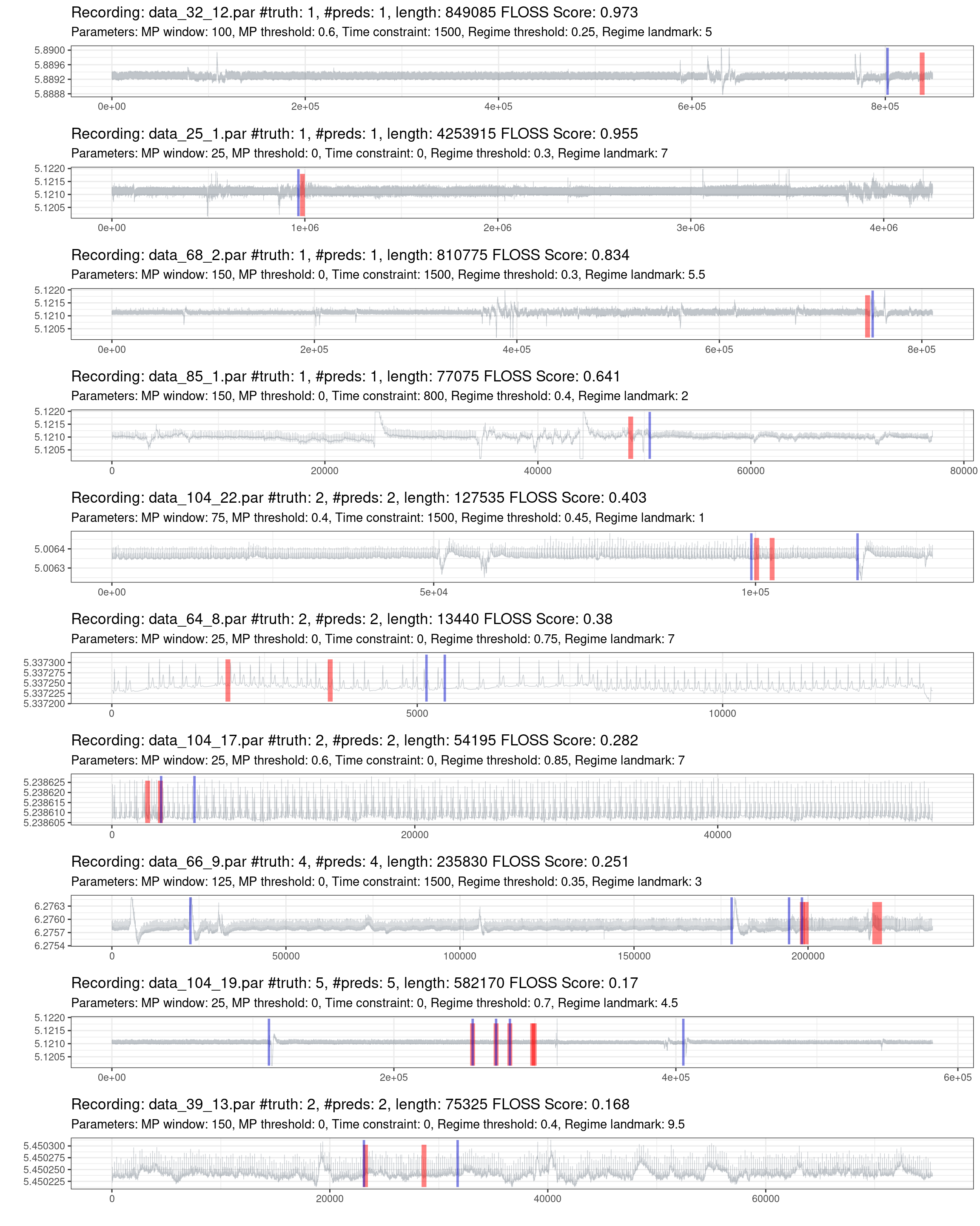
Figure 4.8: Prediction of the worst 10% of recordings (red is the truth, blue are the predictions).
| Version | Author | Date |
|---|---|---|
| 4887954 | Francisco Bischoff | 2023-08-13 |
Fig. 4.9 shows the best performances of the best recordings. Notice that there are recordings with a significant duration and few regime changes, making it hard for a “trivial model” to predict randomly.
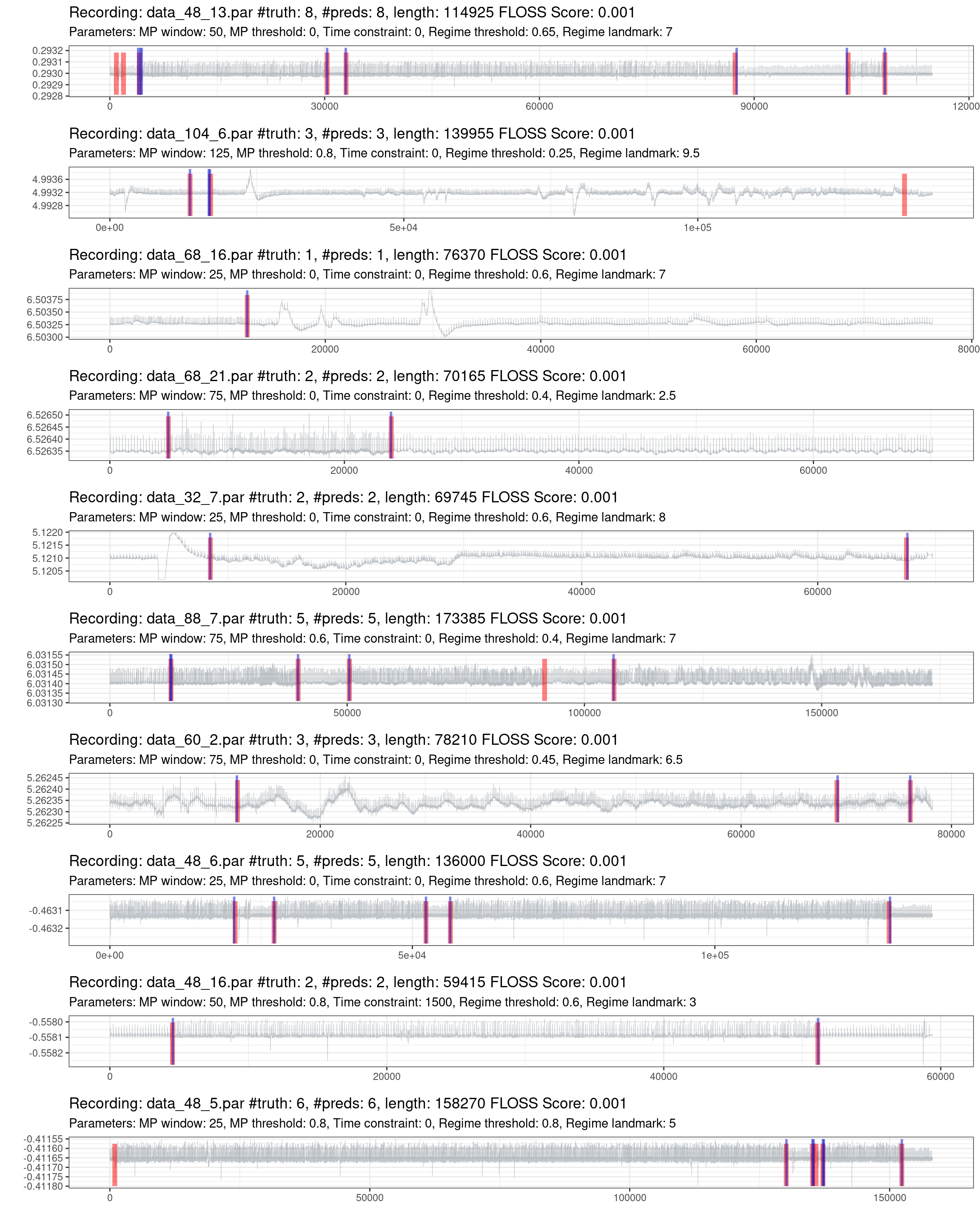
Figure 4.9: Prediction of the best 10% of recordings (red is the truth, blue are the predictions).
| Version | Author | Date |
|---|---|---|
| 4887954 | Francisco Bischoff | 2023-08-13 |
4.1.5.2 By model
Fig. 4.10 shows the distribution of the FLOSS score of the 10% worst (left side) and 10% best models across the recordings (right side). The bluish color highlights the models with SD below 3 and IQR below 1.

Figure 4.10: Violin plot showing the distribution of the FLOSS score achieved by all tested models during the inner ressample. The left half shows the models with the worst performances (10% overall), whereas the right half shows the models with the best performances (10% overall). The models are sorted (left-right) by the mean score (top) and by the median (below). Ties are sorted by the SD and IQR, respectively. The bluish colors highlights models with an SD below 3 and IQR below 1.
| Version | Author | Date |
|---|---|---|
| 4887954 | Francisco Bischoff | 2023-08-13 |
Fig. 4.11 the performance of the six best models. They are ordered from left to right, from the worst record to the best record. The top model is the one with the lowest mean across the scores. The blue line indicates the mean score, and the red line the median score. The scores above 3 are squished in the plot and colored according to the scale in the legend.

Figure 4.11: Performances of the best 6 models across all inner resample of recordings. The recordings are ordered by score, from the worst to the best. Each plot shows one model, starting from the best one. The red line indicates the median score of the model. The blue line indicates the mean score of the model. The gray line limits the zero-score region. The plot is limited on the “y” axis, and the scores above this limit are shown in color.
| Version | Author | Date |
|---|---|---|
| 4887954 | Francisco Bischoff | 2023-08-13 |
4.1.5.3 The Holdout
Finally, Table 4.1 shows a summary of the best five models across all the inner resample (cross-validation). The column mean
shows the average score, and column std_err shows the standard error of the mean. The column holdout shows the
final score of this model on the holdout set (outer resample).
| window_size | regime_threshold | regime_landmark | mean | std_err | holdout |
|---|---|---|---|---|---|
| 150 | 0.45 | 9.0 | 1.08 | 0.49 | 0.66 |
| 150 | 0.35 | 5.0 | 1.10 | 0.57 | 0.80 |
| 100 | 0.50 | 9.5 | 1.10 | 0.48 | 0.62 |
| 125 | 0.45 | 7.5 | 1.11 | 0.55 | 0.57 |
| 125 | 0.45 | 7.0 | 1.11 | 0.54 | 0.61 |
4.2 Classification
As described in section 3.4.5, the classification algorithm is based on the Contrast Profile (CP)48. The CP allows us to detect sequences that at the same time very similar to its neighbors in class A while is very different from the nearest neighbor from class B.
The variables parameters we can tune are the following:
shapelet_size: that we will use interchangeably with the term window_size as is defines the size of the rolling window used to compute the CP. It was used a series of shapelet sizes with exponential distribution, resulting on20values from21to401.top_k: how many shapelets we will select on each CP, being the first one the shapelet with the highest constrast value. It was chosen the default value of10.max_shapelets: the maximum number of shapelets we will allow on selecting the shapelet set. It was set as20to allow more freedom on the selection of shapelets.max_redundance: the maximum number of “redundance” we will allow on selecting the shapelet set. The redundance means more than one shapelet can classify correctly the same observation. It was set as10, to also allow more freedom on the selection of shapelets.
Fig. 4.12 shows the workflow using Nested resamplig as described on 3.4.6.
Figure 4.12: Classification pipeline.
The dataset used for working Classification algorithm was the CinC/Physionet Challenge 2015 was about “Reducing False Arrhythmia Alarms in the ICU22.
The selected records were those that contain ventricular tachycardia. The last 10 seconds (at 250hz) of all records were selected and grouped as TRUE alarm and FALSE alarm. A total of 331 records were used, being 245 FALSE alarms, and 86 TRUE alarms.
The records were split in a proportion of 3/4 (248) for the training set (inner resampling) and 1/4 (83) for the test set (outer resampling). The proportions of TRUE and FALSE alarms were similar to the original dataset: 184 FALSE alarms and 64 TRUE alarms in the training set, and 61 FALSE alarms and 22 TRUE alarms in the test set. The inner resampling was performed using a 5-fold cross-validation.
In order to compute the Contrast Profile (CP), on each fold, the TRUE alarms were concatenated in one single time-series with a small gap of 300 observation of random noise in order to isolate each alarm. The same was done for the FALSE alarms.
The following steps were performed for each fold:
- The CP was computed with several shapelet sizes (from 21 to 401), and top 10 best shapelet candidates were stored based on the CP values.
- Every shapelet candidate was evaluated for the hability to classify as
TRUEorFALSEalarm along all the concatenated time-series.- First, the distance profile of the shapelet was computed against the
FALSEtime-series, and threshold was set in order to not detect anyFALSEalarm asTRUEalarm. - Second, the distance profile of the shapelet was computed against the
TRUEtime-series, and using the threshold computed in the previous step, the number ofTRUEalarms detected was recorded and called the “coverage” of the shapelet.
- First, the distance profile of the shapelet was computed against the
- With this information, a Beam Search was performed in order to select the best set of shapelets that maximize the coverage and minimize the number of shapelets. The set of shapelets may contain shapelets of different sizes.
- The confusion matrix of these sets of shapelets was computed. Other metrics were also computed, such as the F1-score, the accuracy, the precision, the specificity, the MCC, the \(\kappa_m\) and the Kappa.
An example of candidates for ventricular tachycardia is presented on 4.13.

Figure 4.13: Set of shapelets for the classification task. Above shows the model number, the coverage (the proportion of true alarms that were detected) and redundancy during the analysis_split (inner resample), The Precision, the Specificity, and the Km during the testing_split (outer resample).
| Version | Author | Date |
|---|---|---|
| 4887954 | Francisco Bischoff | 2023-08-13 |
After the Inner Resampling is done, the best sets of shapelets are selected and evaluated on the Test Set without retraining a new Contrast Profile. Thus assessing the generalization of the shapelet set on new data.
The criteria to select the best sets of shapelets was described on section 3.5.2 being the Precision the ranking criteria. It was also required that the set being present on more than one fold and in both repetitions. Also, the sets of shapelets that had a negative \(\kappa_m\) were discarded.
The following results were obtained:
| tp | fp | tn | fn | precision | recall | specificity | accuracy | f1 | mcc | km | kappa |
|---|---|---|---|---|---|---|---|---|---|---|---|
| 11 | 1 | 30 | 7 | 0.92 | 0.61 | 0.97 | 0.84 | 0.73 | 0.65 | 0.56 | 0.62 |
| 11 | 1 | 30 | 7 | 0.92 | 0.61 | 0.97 | 0.84 | 0.73 | 0.65 | 0.56 | 0.62 |
| 10 | 1 | 30 | 8 | 0.91 | 0.56 | 0.97 | 0.82 | 0.69 | 0.60 | 0.50 | 0.57 |
| 13 | 2 | 29 | 5 | 0.87 | 0.72 | 0.94 | 0.86 | 0.79 | 0.69 | 0.61 | 0.68 |
| 13 | 3 | 28 | 5 | 0.81 | 0.72 | 0.90 | 0.84 | 0.76 | 0.64 | 0.56 | 0.64 |
| tp | fp | tn | fn | precision | recall | specificity | accuracy | f1 | mcc | km | kappa |
|---|---|---|---|---|---|---|---|---|---|---|---|
| 9 | 3 | 58 | 13 | 0.75 | 0.41 | 0.95 | 0.81 | 0.53 | 0.45 | 0.27 | 0.42 |
| 10 | 1 | 60 | 12 | 0.91 | 0.45 | 0.98 | 0.84 | 0.61 | 0.57 | 0.41 | 0.52 |
| 8 | 5 | 56 | 14 | 0.62 | 0.36 | 0.92 | 0.77 | 0.46 | 0.34 | 0.14 | 0.32 |
| 10 | 3 | 58 | 12 | 0.77 | 0.45 | 0.95 | 0.82 | 0.57 | 0.49 | 0.32 | 0.47 |
| 11 | 5 | 56 | 11 | 0.69 | 0.50 | 0.92 | 0.81 | 0.58 | 0.47 | 0.27 | 0.46 |
| precision | recall | specificity | accuracy | f1_micro | f1_macro | mcc | km | kappa |
|---|---|---|---|---|---|---|---|---|
| 0.75 | 0.46 | 0.95 | 0.81 | 0.72 | 0.55 | 0.47 | 0.27 | 0.46 |
| 0.69 | 0.41 | 0.92 | 0.81 | 0.72 | 0.55 | 0.45 | 0.27 | 0.42 |
| 0.77 | 0.46 | 0.95 | 0.82 | 0.72 | 0.55 | 0.49 | 0.32 | 0.47 |
4.3 Feasibility trial
A side-project called “false.alarm.io” has been derived from this work (an unfortunate mix of “false.alarm” and “PlatformIO”67, the IDE chosen to interface the panoply of embedded systems we can experiment with). The current results of this side-project are very enlightening and show that the final algorithm can indeed be used in small hardware. Further data will be available in the future.
A brief mentioning, linking back to the objectives of this work, an initial trial was done using an ESP32 MCU (Fig. 4.14) in order to be sure if such a small device can handle the task.
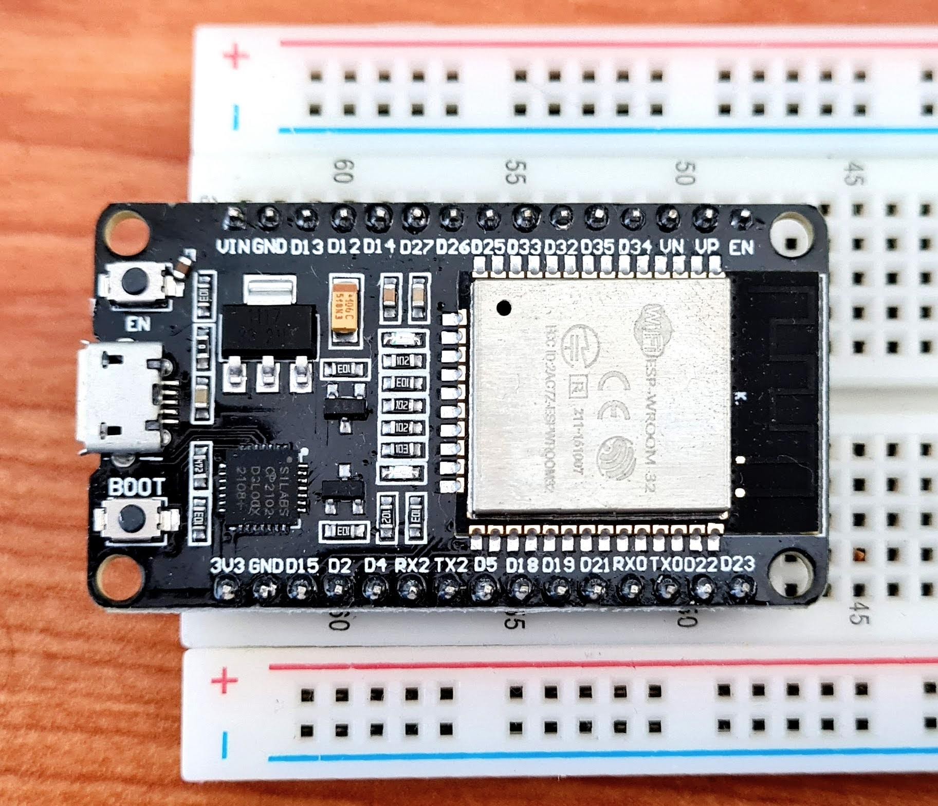
Figure 4.14: ESP32 MCU.
| Version | Author | Date |
|---|---|---|
| 571ac34 | Francisco Bischoff | 2022-01-15 |
Current results show that such device has enough computation power to handle the task in real-time using just one of its two microprocessors. The main limitation seen in advance is the on-chip SRAM that must be well managed.
5 Scientific contributions
5.1 Matrix Profile
Since the first paper that presented this new concept13, many investigations have been made to speed its computation. It is notable how all computations are not dependent on the rolling window size as previous works not using Matrix Profile. Aside from this, we can see that the first STAMP13 algorithm has the time complexity of \(O(n^2log{n})\) while STOMP68 \(O(n^2)\) (a significant improvement), but STOMP lacks the “any-time” property. Later SCRIMP69 solves this problem keeping the same time complexity of \(O(n^2)\). Here we are in the “exact” algorithms domain, and we will not extend the scope for conciseness.
The main issue with the algorithms above is the dependency on a fast Fourier transform (FFT) library. FFT has been extensively optimized and architecture/CPU bounded to exploit the most of speed. Also, padding data to some power of 2 happens to increase the algorithm’s efficiency. We can argue that time complexity doesn’t mean “faster” when we can exploit low-level instructions. In our case, using FFT in a low-power device is overkilling. For example, a quick search over the internet gives us a hint that computing FFT on 4096 data in an ESP32 takes about 21ms (~47 computations in 1 second). This means ~79 seconds for computing all FFT’s (~3797) required for STAMP using a window of 300. Currently, we can compute a full matrix of 5k data in about 9 seconds in an ESP32 MCU (Fig. 4.14), and keep updating it as fast as 1 min of data (at 250hz) in just 6 seconds.
Recent works using exact algorithms are using an unpublished algorithm called MPX, which computes the Matrix Profile using cross-correlation methods ending up faster and is easily portable.
On computing the Matrix Profile: the contribution of this work on this area is adding the Online capability to MPX, which means we can update the Matrix Profile as new data comes in.
On extending the Matrix Profile: the contribution of this work on this area is the use of an unexplored constraint that we could apply on building the Matrix Profile we are calling Similarity Threshold (ST). The original work outputs the similarity values in Euclidean Distance (ED) values, while MPX naturally outputs the Pearson’s correlation coefficients (CC) values. Both ED and CC are interchangeable using the Equation \(\eqref{edcc}\). However, we may argue that it is easier to compare values that do not depend on the window size during an exploratory phase. MPX happens to naturally return values in CC, saving a few more computation time. The ST is an interesting factor that we can use, especially when detecting pattern changes during time. The FLOSS algorithm relies on counting references between indexes in the time series. ST can help remove “noise” from these references since only similar patterns above a certain threshold are referenced, and changes have more impact on these counts. The best ST threshold is still to be determined.
\[
CC = 1 - \frac{ED}{(2 \times WindowSize)} \tag{9} \label{edcc}
\]
5.2 Regime change detection
In the original paper, in chapter 3.5, the authors of FLOSS wisely introduce the temporal constraint, which improves the sensitivity of regime change detection on situations where a regime may alternate in short periods.
Nevertheless, the authors declare the correction curve typically used on the algorithm as “simply a uniform distribution”, but this is not an accurate statement. The Arc Counts of newly incoming data is truncated by the same amount of temporal constraint. This prevents detecting a regime change in the last 10 seconds completely, as this thesis requires.
The main contribution of this work in this area is overcoming this issue by computing the theoretical distribution using the temporal constraint parameters beforehand. as shown in Fig. 5.1. That gives us enough data to evaluate a regime change accurately utilizing a minimum of \(2 \times WindowSize\) datapoints.

Figure 5.1: 1D-IAC distributions for earlier temporal constraint (on Matrix Profile).
6 Scientific outcomes
This research has already yielded two R packages concerning the MP algorithms from UCR17. The
first package is called tsmp, and a paper was also published in the R Journal18
(Journal Impact Factor™, 2020 of 3.984). The second package is called matrixprofiler and enhances
the first one, using low-level language to improve computational speed. The author has also joined
the Matrix Profile Foundation is a co-founder with contributors from Python and Go languages19,20. The benchmarks of the R implementation are available online70.
Additionally to the above publication and the publication of the ongoing literature survey, two articles about this thesis subject will be published. The first regards the application of the FLOSS algorithm on real-time ECG showing its potential on using on low-power devices. The second is regarding the use of combined shapelets for relevant ECG patterns identification.
7 Expected results and outcomes
In the end, this thesis will provide a framework for identifying life-threatening conditions using biological streaming data on devices with low CPU and low memory specifications. We expect to achieve a high-quality model on identifying these pathological conditions maintaining their robustness in the presence of noise and artifacts seen on real-world applications.
8 References
─ Session info ───────────────────────────────────────────────────────────────
 setting  value
 version  R version 4.3.1 (2023-06-16)
 os       Ubuntu 22.04.2 LTS
 system   x86_64, linux-gnu
 ui       X11
 language (EN)
 collate  en_US.UTF-8
 ctype    en_US.UTF-8
 tz       Europe/Lisbon
 date     2023-08-13
 pandoc   2.17.0.1 @ /usr/bin/ (via rmarkdown)

─ Packages ───────────────────────────────────────────────────────────────────
 package      * version     date (UTC) lib source
 askpass        1.1         2019-01-13 [1] CRAN (R 4.3.0)
 backports      1.4.1       2021-12-13 [1] CRAN (R 4.3.1)
 base64url      1.4         2018-05-14 [1] CRAN (R 4.3.0)
 bit            4.0.5       2022-11-15 [1] CRAN (R 4.3.0)
 bit64          4.0.5       2020-08-30 [1] CRAN (R 4.3.0)
 bookdown       0.35.1      2023-08-13 [1] Github (rstudio/bookdown@661567e)
 bslib          0.5.1       2023-08-11 [1] CRAN (R 4.3.1)
 cachem         1.0.8       2023-05-01 [1] CRAN (R 4.3.0)
 callr          3.7.3       2022-11-02 [1] CRAN (R 4.3.1)
 checkmate      2.2.0       2023-04-27 [1] CRAN (R 4.3.0)
 class          7.3-22      2023-05-03 [2] CRAN (R 4.3.1)
 cli            3.6.1       2023-03-23 [1] CRAN (R 4.3.1)
 codetools      0.2-19      2023-02-01 [2] CRAN (R 4.3.0)
 colorspace     2.1-0       2023-01-23 [1] CRAN (R 4.3.0)
 crayon         1.5.2       2022-09-29 [1] CRAN (R 4.3.1)
 credentials    1.3.2       2021-11-29 [1] CRAN (R 4.3.0)
 data.table     1.14.8      2023-02-17 [1] CRAN (R 4.3.0)
 debugme        1.1.0       2017-10-22 [1] CRAN (R 4.3.0)
 devtools       2.4.5       2022-10-11 [1] CRAN (R 4.3.0)
 dials          1.2.0       2023-04-03 [1] CRAN (R 4.3.0)
 DiceDesign     1.9         2021-02-13 [1] CRAN (R 4.3.0)
 digest         0.6.33      2023-07-07 [1] CRAN (R 4.3.1)
 dplyr          1.1.2       2023-04-20 [1] CRAN (R 4.3.0)
 ellipsis       0.3.2       2021-04-29 [1] CRAN (R 4.3.0)
 evaluate       0.21        2023-05-05 [1] CRAN (R 4.3.0)
 fansi          1.0.4       2023-01-22 [1] CRAN (R 4.3.0)
 farver         2.1.1       2022-07-06 [1] CRAN (R 4.3.0)
 fastmap        1.1.1       2023-02-24 [1] CRAN (R 4.3.0)
 forcats        1.0.0       2023-01-29 [1] CRAN (R 4.3.0)
 foreach        1.5.2       2022-02-02 [1] CRAN (R 4.3.0)
 fs             1.6.3       2023-07-20 [1] CRAN (R 4.3.1)
 furrr          0.3.1       2022-08-15 [1] CRAN (R 4.3.0)
 future         1.33.0      2023-07-01 [1] CRAN (R 4.3.1)
 future.apply   1.11.0      2023-05-21 [1] CRAN (R 4.3.1)
 future.callr   0.8.2       2023-08-09 [1] CRAN (R 4.3.1)
 generics       0.1.3       2022-07-05 [1] CRAN (R 4.3.0)
 gert           1.9.3       2023-08-07 [1] CRAN (R 4.3.1)
 getPass        0.2-2       2017-07-21 [1] CRAN (R 4.3.0)
 ggplot2      * 3.4.2       2023-04-03 [1] CRAN (R 4.3.0)
 git2r          0.32.0.9000 2023-06-30 [1] Github (ropensci/git2r@9c42d41)
 gittargets   * 0.0.6.9000  2023-05-05 [1] Github (wlandau/gittargets@2d448ff)
 globals        0.16.2      2022-11-21 [1] CRAN (R 4.3.0)
 glue         * 1.6.2       2022-02-24 [1] CRAN (R 4.3.1)
 gower          1.0.1       2022-12-22 [1] CRAN (R 4.3.0)
 GPfit          1.0-8       2019-02-08 [1] CRAN (R 4.3.0)
 gridExtra      2.3         2017-09-09 [1] CRAN (R 4.3.0)
 gtable         0.3.3       2023-03-21 [1] CRAN (R 4.3.0)
 hardhat        1.3.0       2023-03-30 [1] CRAN (R 4.3.0)
 here         * 1.0.1       2020-12-13 [1] CRAN (R 4.3.0)
 highr          0.10        2022-12-22 [1] CRAN (R 4.3.1)
 hms            1.1.3       2023-03-21 [1] CRAN (R 4.3.0)
 htmltools      0.5.6       2023-08-10 [1] CRAN (R 4.3.1)
 htmlwidgets    1.6.2       2023-03-17 [1] CRAN (R 4.3.0)
 httpuv         1.6.11      2023-05-11 [1] CRAN (R 4.3.1)
 httr           1.4.6       2023-05-08 [1] CRAN (R 4.3.1)
 igraph         1.5.1       2023-08-10 [1] CRAN (R 4.3.1)
 ipred          0.9-14      2023-03-09 [1] CRAN (R 4.3.0)
 iterators      1.0.14      2022-02-05 [1] CRAN (R 4.3.0)
 jquerylib      0.1.4       2021-04-26 [1] CRAN (R 4.3.0)
 jsonlite       1.8.7       2023-06-29 [1] CRAN (R 4.3.0)
 kableExtra   * 1.3.4       2021-02-20 [1] CRAN (R 4.3.0)
 knitr          1.43        2023-05-25 [1] CRAN (R 4.3.0)
 labeling       0.4.2       2020-10-20 [1] CRAN (R 4.3.0)
 later          1.3.1       2023-05-02 [1] CRAN (R 4.3.1)
 lattice        0.21-8      2023-04-05 [2] CRAN (R 4.3.0)
 lava           1.7.2.1     2023-02-27 [1] CRAN (R 4.3.0)
 lhs            1.1.6       2022-12-17 [1] CRAN (R 4.3.0)
 lifecycle      1.0.3       2022-10-07 [1] CRAN (R 4.3.1)
 listenv        0.9.0       2022-12-16 [1] CRAN (R 4.3.0)
 lubridate      1.9.2       2023-02-10 [1] CRAN (R 4.3.0)
 magrittr       2.0.3       2022-03-30 [1] CRAN (R 4.3.1)
 MASS           7.3-60      2023-05-04 [2] CRAN (R 4.3.1)
 Matrix         1.6-0       2023-07-08 [1] CRAN (R 4.3.1)
 memoise        2.0.1       2021-11-26 [1] CRAN (R 4.3.0)
 mgcv           1.9-0       2023-07-11 [1] CRAN (R 4.3.1)
 mime           0.12        2021-09-28 [1] CRAN (R 4.3.0)
 miniUI         0.1.1.1     2018-05-18 [1] CRAN (R 4.3.0)
 munsell        0.5.0       2018-06-12 [1] CRAN (R 4.3.0)
 nlme           3.1-163     2023-08-09 [1] CRAN (R 4.3.1)
 nnet           7.3-19      2023-05-03 [2] CRAN (R 4.3.1)
 openssl        2.1.0       2023-07-15 [1] CRAN (R 4.3.1)
 parallelly     1.36.0      2023-05-26 [1] CRAN (R 4.3.1)
 parsnip        1.1.0       2023-04-12 [1] CRAN (R 4.3.0)
 patchwork    * 1.1.2       2022-08-19 [1] CRAN (R 4.3.0)
 pillar         1.9.0       2023-03-22 [1] CRAN (R 4.3.0)
 pkgbuild       1.4.2       2023-06-26 [1] CRAN (R 4.3.1)
 pkgconfig      2.0.3       2019-09-22 [1] CRAN (R 4.3.0)
 pkgload        1.3.2.1     2023-07-08 [1] CRAN (R 4.3.1)
 prettyunits    1.1.1       2020-01-24 [1] CRAN (R 4.3.0)
 processx       3.8.2       2023-06-30 [1] CRAN (R 4.3.1)
 prodlim        2023.03.31  2023-04-02 [1] CRAN (R 4.3.0)
 profvis        0.3.8       2023-05-02 [1] CRAN (R 4.3.1)
 promises       1.2.1       2023-08-10 [1] CRAN (R 4.3.1)
 ps             1.7.5       2023-04-18 [1] CRAN (R 4.3.1)
 purrr          1.0.2       2023-08-10 [1] CRAN (R 4.3.1)
 R6             2.5.1       2021-08-19 [1] CRAN (R 4.3.1)
 Rcpp           1.0.11      2023-07-06 [1] CRAN (R 4.3.1)
 RcppParallel   5.1.7       2023-02-27 [1] CRAN (R 4.3.0)
 readr          2.1.4       2023-02-10 [1] CRAN (R 4.3.0)
 recipes        1.0.7       2023-08-10 [1] CRAN (R 4.3.1)
 remotes        2.4.2.1     2023-07-18 [1] CRAN (R 4.3.1)
 renv           0.17.3      2023-04-06 [1] CRAN (R 4.3.1)
 rlang          1.1.1       2023-04-28 [1] CRAN (R 4.3.0)
 rmarkdown      2.23.4      2023-08-13 [1] Github (rstudio/rmarkdown@054d735)
 rpart          4.1.19      2022-10-21 [2] CRAN (R 4.3.0)
 rprojroot      2.0.3       2022-04-02 [1] CRAN (R 4.3.1)
 rsample        1.1.1       2022-12-07 [1] CRAN (R 4.3.0)
 rstudioapi     0.15.0      2023-07-07 [1] CRAN (R 4.3.1)
 rvest          1.0.3       2022-08-19 [1] CRAN (R 4.3.0)
 sass           0.4.7       2023-07-15 [1] CRAN (R 4.3.1)
 scales         1.2.1       2022-08-20 [1] CRAN (R 4.3.0)
 sessioninfo    1.2.2       2021-12-06 [1] CRAN (R 4.3.0)
 shapviz        0.9.1       2023-07-18 [1] CRAN (R 4.3.1)
 shiny          1.7.5       2023-08-12 [1] CRAN (R 4.3.1)
 signal         0.7-7       2021-05-25 [1] CRAN (R 4.3.0)
 stringi        1.7.12      2023-01-11 [1] CRAN (R 4.3.1)
 stringr        1.5.0       2022-12-02 [1] CRAN (R 4.3.1)
 survival       3.5-5       2023-03-12 [2] CRAN (R 4.3.1)
 svglite        2.1.1.9000  2023-05-05 [1] Github (r-lib/svglite@6c1d359)
 sys            3.4.2       2023-05-23 [1] CRAN (R 4.3.1)
 systemfonts    1.0.4       2022-02-11 [1] CRAN (R 4.3.0)
 tarchetypes  * 0.7.7       2023-06-15 [1] CRAN (R 4.3.1)
 targets      * 1.2.2       2023-08-10 [1] CRAN (R 4.3.1)
 tibble       * 3.2.1       2023-03-20 [1] CRAN (R 4.3.0)
 tidyr          1.3.0       2023-01-24 [1] CRAN (R 4.3.0)
 tidyselect     1.2.0       2022-10-10 [1] CRAN (R 4.3.0)
 timechange     0.2.0       2023-01-11 [1] CRAN (R 4.3.0)
 timeDate       4022.108    2023-01-07 [1] CRAN (R 4.3.0)
 timetk         2.8.3       2023-03-30 [1] CRAN (R 4.3.0)
 tsmp           0.4.15      2022-08-20 [1] CRAN (R 4.3.0)
 tune           1.1.1       2023-04-11 [1] CRAN (R 4.3.0)
 tzdb           0.4.0       2023-05-12 [1] CRAN (R 4.3.1)
 urlchecker     1.0.1       2021-11-30 [1] CRAN (R 4.3.0)
 usethis        2.2.2.9000  2023-07-17 [1] Github (r-lib/usethis@467ff57)
 utf8           1.2.3       2023-01-31 [1] CRAN (R 4.3.0)
 uuid           1.1-0       2022-04-19 [1] CRAN (R 4.3.0)
 vctrs          0.6.3       2023-06-14 [1] CRAN (R 4.3.1)
 viridisLite    0.4.2       2023-05-02 [1] CRAN (R 4.3.1)
 visNetwork   * 2.1.2       2022-09-29 [1] CRAN (R 4.3.0)
 vroom          1.6.3       2023-04-28 [1] CRAN (R 4.3.1)
 webshot        0.5.5       2023-06-26 [1] CRAN (R 4.3.1)
 whisker        0.4.1       2022-12-05 [1] CRAN (R 4.3.0)
 withr          2.5.0       2022-03-03 [1] CRAN (R 4.3.1)
 workflowr    * 1.7.0       2021-12-21 [1] CRAN (R 4.3.0)
 workflows      1.1.3       2023-02-22 [1] CRAN (R 4.3.0)
 xfun           0.40        2023-08-09 [1] CRAN (R 4.3.1)
 xgboost        1.7.5.1     2023-03-30 [1] CRAN (R 4.3.0)
 xml2           1.3.5       2023-07-06 [1] CRAN (R 4.3.1)
 xtable         1.8-4       2019-04-21 [1] CRAN (R 4.3.0)
 xts            0.13.1      2023-04-16 [1] CRAN (R 4.3.0)
 yaml           2.3.7       2023-01-23 [1] CRAN (R 4.3.1)
 yardstick      1.0.0.9000  2023-05-25 [1] Github (tidymodels/yardstick@90ab794)
 zoo            1.8-12      2023-04-13 [1] CRAN (R 4.3.0)

 [1] /workspace/.cache/R/renv/proj_libs/false.alarm-d6f1a0d1/R-4.3/x86_64-pc-linux-gnu
 [2] /usr/lib/R/library

──────────────────────────────────────────────────────────────────────────────