Regime changes 2.0
Francisco Bischoff
on January 02, 2024
Last updated: 2024-01-02
Checks: 7 0
Knit directory:
develop/docs/
This reproducible R Markdown analysis was created with workflowr (version 1.7.0). The Checks tab describes the reproducibility checks that were applied when the results were created. The Past versions tab lists the development history.
Great! Since the R Markdown file has been committed to the Git repository, you know the exact version of the code that produced these results.
Great job! The global environment was empty. Objects defined in the global environment can affect the analysis in your R Markdown file in unknown ways. For reproduciblity it’s best to always run the code in an empty environment.
The command set.seed(20201020) was run prior to running the code in the R Markdown file.
Setting a seed ensures that any results that rely on randomness, e.g.
subsampling or permutations, are reproducible.
Great job! Recording the operating system, R version, and package versions is critical for reproducibility.
Nice! There were no cached chunks for this analysis, so you can be confident that you successfully produced the results during this run.
Great job! Using relative paths to the files within your workflowr project makes it easier to run your code on other machines.
Great! You are using Git for version control. Tracking code development and connecting the code version to the results is critical for reproducibility.
The results in this page were generated with repository version dc13c05. See the Past versions tab to see a history of the changes made to the R Markdown and HTML files.
Note that you need to be careful to ensure that all relevant files for the
analysis have been committed to Git prior to generating the results (you can
use wflow_publish or wflow_git_commit). workflowr only
checks the R Markdown file, but you know if there are other scripts or data
files that it depends on. Below is the status of the Git repository when the
results were generated:
Ignored files:
    Ignored:    .Renviron
    Ignored:    .Rhistory
    Ignored:    .docker/
    Ignored:    .luarc.json
    Ignored:    analysis/shiny/rsconnect/
    Ignored:    analysis/shiny_land/rsconnect/
    Ignored:    analysis/shiny_ventricular/rsconnect/
    Ignored:    analysis/shiny_vtachy/rsconnect/
    Ignored:    dev/
    Ignored:    inst/extdata/
    Ignored:    renv/staging/
    Ignored:    tmp/
Note that any generated files, e.g. HTML, png, CSS, etc., are not included in this status report because it is ok for generated content to have uncommitted changes.
These are the previous versions of the repository in which changes were made
to the R Markdown (analysis/regime_optimize_2.Rmd) and HTML (docs/regime_optimize_2.html)
files. If you’ve configured a remote Git repository (see
?wflow_git_remote), click on the hyperlinks in the table below to
view the files as they were in that past version.
| File | Version | Author | Date | Message |
|---|---|---|---|---|
| Rmd | dc13c05 | Francisco Bischoff | 2024-01-02 | Refine predictive model and significance |
| html | b149bf4 | Francisco Bischoff | 2023-10-10 | re-rendered |
| Rmd | ce66066 | Francisco Bischoff | 2023-10-10 | fixed lmk |
| Rmd | 5636465 | Francisco Bischoff | 2023-10-05 | regime 2 wip |
| html | 5636465 | Francisco Bischoff | 2023-10-05 | regime 2 wip |
| html | d06c64f | Francisco Bischoff | 2022-10-09 | Squashed commit of the following: |
| html | f9f551d | Francisco Bischoff | 2022-10-06 | Build site. |
| Rmd | 6b7a6c7 | Francisco Bischoff | 2022-10-06 | PR done |
| Rmd | dbbd1d6 | Francisco Bischoff | 2022-08-22 | Squashed commit of the following: |
| html | dbbd1d6 | Francisco Bischoff | 2022-08-22 | Squashed commit of the following: |
| Rmd | de21180 | Francisco Bischoff | 2022-08-21 | Squashed commit of the following: |
| html | de21180 | Francisco Bischoff | 2022-08-21 | Squashed commit of the following: |
1 Regime changes optimization (continuation)
Following the previous article, this article aims to complete the analysis of the regime change optimization. Here we add the regime_landmark parameter to the optimization.
1.1 Current pipeline
Figure 1.1: FLOSS pipeline.
1.2 Tuning process
As we have seen previously, the FLOSS algorithm is built on top of the Matrix Profile (MP). Thus, we have proposed several parameters that may or not impact the FLOSS prediction performance.
The variables for building the MP are:
mp_threshold: the minimum similarity value to be considered for 1-NN.time_constraint: the maximum distance to look for the nearest neighbor.window_size: the default parameter always used to build an MP.
Later, the FLOSS algorithm also has a parameter that needs tuning to optimize the prediction:
regime_threshold: the threshold below which a regime change is considered.regime_landmark: the point in time where the regime threshold is applied.
Using the tidymodels framework, we performed a basic grid search on all these parameters, now limiting the exploration
on the MP and focusing on the FLOSS parameters.
The workflow is as follows:
- From the original set of 229 records, a subset of 137 records was selected for the grid search.
- The MP parameters were explored using the following values:
mp_threshold: 0.0, 0.4, 0.6 and 0.8;time_constraint: 0, 800 and 1500;window_size: 25, 50, 75, 100, 125 and 150;
- The FLOSS parameters were explored using the following values:
regime_threshold: 0.05 to 0.90, by 0.05 steps;regime_landmark: 1 to 10, by 0.5 steps.
The results were then combined with the previous optimization and deduplicated.
1.3 Parameters analysis
As before, we started by computing the importance of each parameter1. We used the same approach using the Bayesian Additive Regression Trees (BART) model to fit the tuning parameters as predictors of the FLOSS score.
1.3.1 Interactions
Before starting the parameter importance analysis, we need to consider the parameter interactions since this is usually the weak spot of the analysis techniques.
The first BART model was fitted using the following parameters:
\[\begin{equation} \begin{aligned} E( score ) &= \alpha + time\_constraint\\ &\quad + mp\_threshold + window\_size\\ &\quad + regime\_threshold + regime\_landmark \end{aligned} \tag{1.1} \end{equation}\]
After checking the interactions, this is the refitted model:
\[\begin{equation} \begin{aligned} E( score ) &= \alpha + time\_constraint\\ &\quad + mp\_threshold + window\_size\\ &\quad + regime\_threshold + regime\_landmark\\ &\quad + \left(time\_constraint \times regime\_landmark\right)\\ &\quad + \left(time\_constraint \times regime\_threshold\right) \end{aligned} \tag{1.2} \end{equation}\]
Fig. 1.2 shows the variable interaction strength between pairs of variables. That allows us to
verify if there are any significant interactions between the variables. Using the information from the first model fit,
equation (1.1), we see that time_constraint interacts strongly with regime_landmark and regime_threshold.
Also it seems that regime_landmark and regime_threshold interacts strongly with each other.
Knowing how the model is built, we already can antecipate that the regime_landmark can indeed have a strong relation
with regime_threshold since the landmark is the point in time where the threshold is applied.
This is not a problem per se but a signal we must be aware of when exploring the parameters.
In order to explore the interactions, we chose to refit the model adding the first two interactions, equation (1.2).
Here we see at the lower plot of Fig. 1.2 that accounting for these interactions, the global strength of
the variables visibly changes, with regime_landmark and regime_threshold losing strength.
![Variable interactions strength using feature importance ranking measure (FIRM) approach [@Greenwell2018]. A) Shows strong interaction between `time_constraint` and `regime_landmark` and `regime_threshold`. Also we see a expected strong interaction between `regime_landmark` and `regime_threshold`. B) Refitting the model with the first two interactions taken into account, the overall strength is substantially changed, notably for `regime_landmark` and `regime_threshold`.](figure/regime_optimize_2.Rmd/interaction-1.svg)
Figure 1.2: Variable interactions strength using feature importance ranking measure (FIRM) approach2. A) Shows strong interaction between time_constraint and regime_landmark and regime_threshold. Also we see a expected strong interaction between regime_landmark and regime_threshold. B) Refitting the model with the first two interactions taken into account, the overall strength is substantially changed, notably for regime_landmark and regime_threshold.
1.3.2 Importance
After evaluating the interactions, we can then perform the analysis of the variable importance. The goal is to understand how the FLOSS score behaves when we change the parameters.
The techniques for evaluating the variable importances were described in the previous article.
1.3.3 Importance analysis
Using the three techniques simultaneously allows a broad comparison of the model behavior3. All three methods are model-agnostic (separates interpretation from the model), but as we have seen, each method has its advantages and disadvantages4.
Fig. 1.3 then shows the variable importance using three methods: Feature Importance Ranking Measure (FIRM) using Individual Conditional Expectation (ICE), Permutation-based, and Shapley Additive explanations (SHAP). The first line shows the original fit, and the second line shows the refit, taking into account the interactions.
Interestingly, the three methods agree with each other, and the interactions didn’t change the overall importance of the variables. This can probably be explained by the magnitude of the x-axis, which may lead us to overestimate the importance of the interactions in this model since there is no formal threshold for saying that an interaction is important or not.

Figure 1.3: Variables importances using three different methods. A) Feature Importance Ranking Measure using ICE curves. B) Permutation method (100x). C) SHAP (100 iterations). Line 1 refers to the original fit, and line 2 to the re-fit, taking into account the interactions between variables (Fig. 1.2). Notice that all methods agree with each other, and the interactions didn’t change the overall importance of the variables.
Fig. 1.4 and 1.5 show the effect of each feature on the FLOSS score. The
more evident difference is the shape of the effect of time_constraint which we will delve carefully below.
Notice however that the refitted model produces a cleaner plot in Fig. 1.5.
Based on Figures 1.3 and 1.5 we can infer that:
regime_landmark: is the “second” most important feature, however it shows a clear interaction with theregime_thresholdif we look at the color scale, so both must be tuned simultaneously. In both plots, it seems to improve the model score when landmark is <5.0s.regime_threshold: seems not as important as theregime_landmark,but since there is a high interaction, it must not be underestimated, and by prior knowledge we understand that there must be some kind of threshold to mark a regime change.window_size: has a low importance. Nevertheless, it seems to have an optimal value, around 80-120 In this setting, the model is being tuned towards the changes from atrial fibrillation/non-fibrillation; thus, the “shape of interest” is small compared to the whole heartbeat waveform. As Beyer et al. noted, “as dimensionality increases, the distance to the nearest data point approaches the distance to the farthest data point”5, which means that the bigger the window size, the smaller will be the contrast between different regimesm, thus the final objective of the model may influence the optimal window size.mp_threshold: has the lowest impact on the score, and the plot shows that this parameter has virtually no influence on the model performance.time_constraint: is a parameter that must be interpreted cautiously. The 0 (zero) value means no constraint, which is equivalent to the size of the FLOSS history buffer (in our setting, 5000). This allows us to understand that the model doesn’t need this paramenter, and further adjusts in performance can be achieved by setting the size of the history buffer.
In short, for the MP computation (the most expensive in terms of complexity), the parameter that is worth tuning
is only the window_size, while for the FLOSS computation, both regime_threshold (mainly) and regime_landmark
shall be tuned.

Figure 1.4: This shows the Shapley value distribution for each variable. Smaller values means a better FLOSS score since “zero” is a perfect prediction. This plot doesn’t take into account the variable interactions.

Figure 1.5: This shows the Shapley value distribution for each variable. Smaller values means a better FLOSS score since “zero” is a perfect prediction. This plot is taking into account the variable interactions, which appears to result in a cleaner plot.
According to the FLOSS paper6, the window_size is indeed a feature that can be tuned; nevertheless,
the results appear to be similar in a reasonably wide range of window sizes, up to a limit, consistent with our findings.
1.4 Visualizing the predictions
At this point, the grid search tested a total of 23,389 models with resulting (individual) scores from 0.0002 to 1669.83 (Q25: 0.9838, Q50: 1.8093, Q75: 3.3890).
1.4.1 By recording
First, we will visualize how the models (in general) performed throughout the individual recordings.
Fig. 1.6 shows a violin plot of equal areas clipped to the minimum value. The blue color indicates the recordings with a small IQR (interquartile range) of model scores. We see on the left half 10% of the recordings with the worst minimum score, and on the right half, 10% of the recordings with the best minimum score.
Next, we will visualize some of these predictions to understand why some recordings were difficult to segment. For us to have a simple baseline: a recording with just one regime change, and the model predicts exactly one regime change, but far from the truth, the score will be roughly 1.

Figure 1.6: Violin plot showing the distribution of the FLOSS score achieved by all tested models by recording. The left half shows the recordings that were difficult to predict (10% overall), whereas the right half shows the recordings that at least one model could achieve a good prediction (10% overall). The recordings are sorted (left-right) by the minimum (best) score achieved in descending order, and ties are sorted by the median of all recording scores. The blue color highlights recordings where models had an IQR variability of less than one. As a simple example, a recording with just one regime change, and the model predicts exactly one change, far from the truth, the score will be roughly 1.
Fig. 1.7 shows the best effort in predicting the most complex recordings. One information not declared before is that if the model does not predict any change, it will put a mark on the zero position. On the other side, the truth markers positioned at the beginning and the end of the recording were removed, as these locations lack information and do not represent a streaming setting. Compared to the corresponding figure in the previous article, we can see that even the most complex recordings had better predictions.
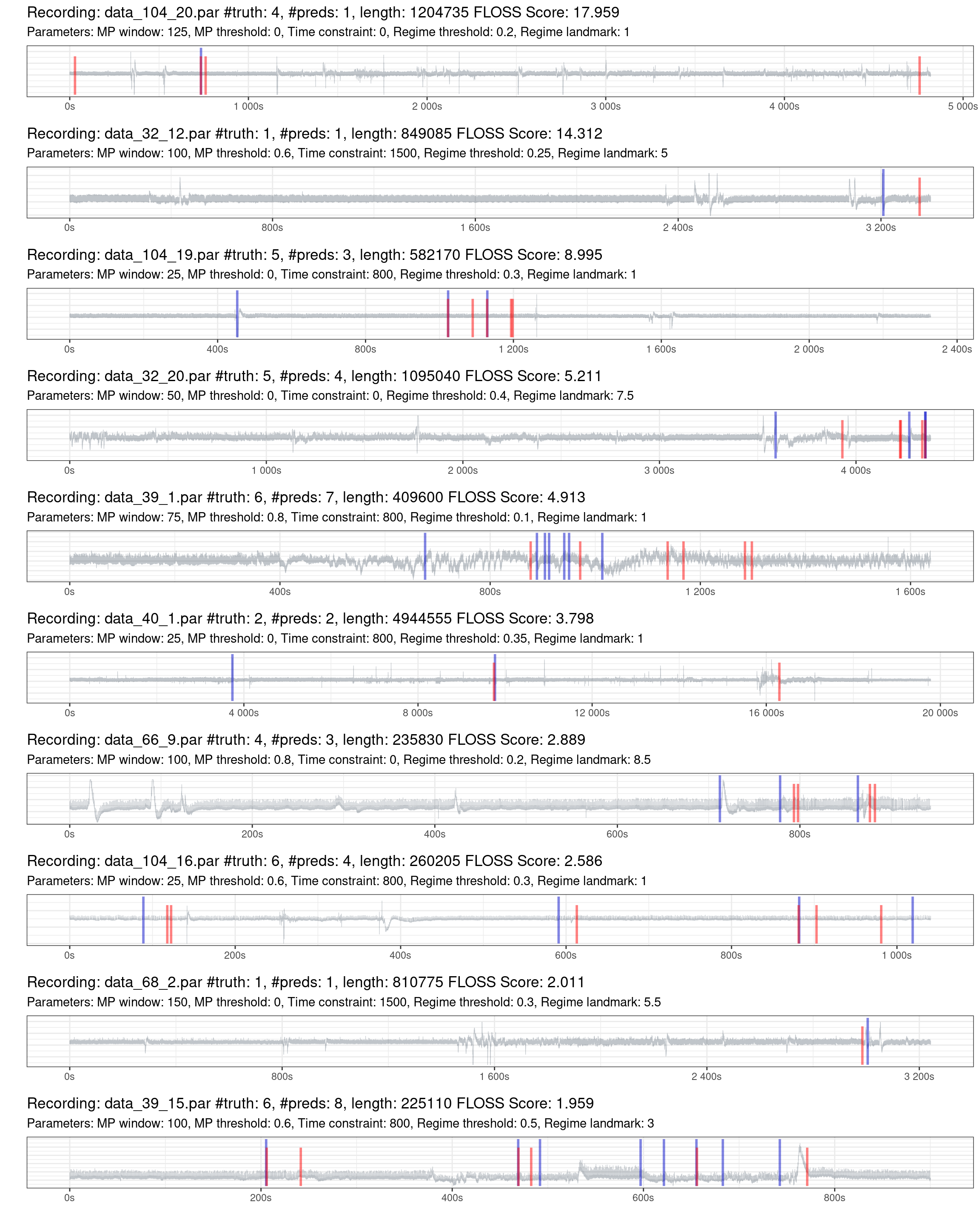
Figure 1.7: Prediction of the worst 10% of recordings (red is the truth, blue are the predictions).
Fig. 1.8 shows the best performances of the best recordings. Notice that there are recordings with a significant duration and few regime changes, making it hard for a “trivial model” to predict randomly.
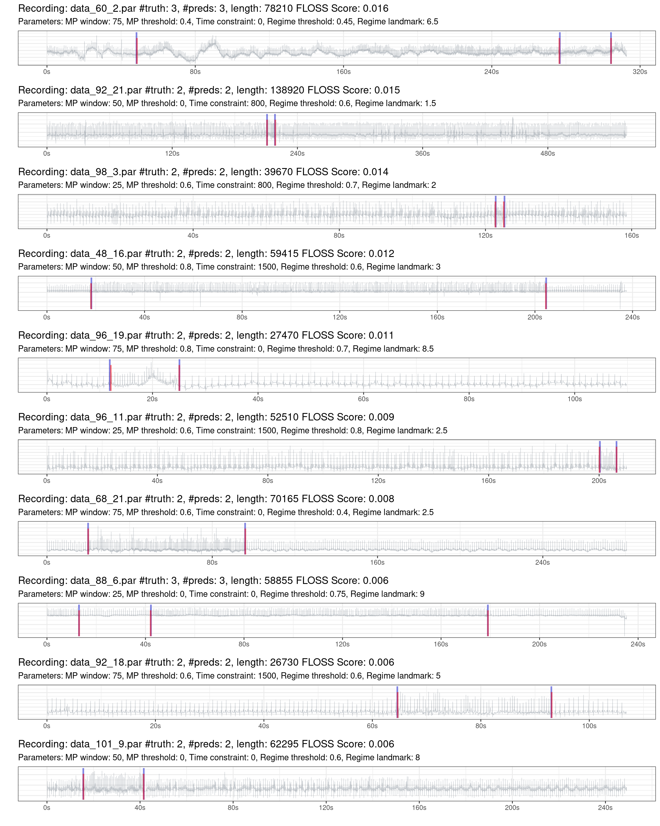
Figure 1.8: Prediction of the best 10% of recordings (red is the truth, blue are the predictions).
An online interactive version of all the datasets and predictions can be accessed at Shiny app.
1.4.2 By model
Fig. 1.9 shows the distribution of the FLOSS score of the 10% worst (left side) and 10% best models across the recordings (right side). The bluish color highlights the models with SD below 3 and IQR below 1.
Here again, we can compare with the previous article and see an improvement in the performance, as the models present lower SD and IQR.

Figure 1.9: Violin plot showing the distribution of the FLOSS score achieved by all tested models during the inner ressample. The left half shows the models with the worst performances (10% overall), whereas the right half shows the models with the best performances (10% overall). The models are sorted (left-right) by the mean score (top) and by the median (below). Ties are sorted by the SD and IQR, respectively. The bluish colors highlights models with an SD below 3 and IQR below 1.
Fig. 1.10 the performance of the six best models. They are ordered from left to right, from the worst record to the best record. The top model is the one with the lowest mean across the scores. The red line indicates the median score. The scores above 3 are squished in the plot and colored according to the scale in the legend. Notice the improvement on the blue and red lines compared to the previous article.

Figure 1.10: Performances of the best 6 models across all inner resample of recordings. The recordings are ordered by score, from the worst to the best. Each plot shows one model, starting from the best one. The red line indicates the median score of the model. The gray line limits the zero-score region. The plot is limited on the “y” axis, and the scores above this limit are shown in color.
We can see that some records (namely #19, #41, #93, #100, #107) are contained in the set of “difficult” records shown in Fig. 1.6.
2 Current status
The current status of the project shows that FLOSS is up to the task of signaling possible regime changes.
After introducing the regime_landmark feature, the performance improves significantly, and we can narrow down the tuning space to a small number of parameters.
In parallel, another score measure is being developed based on the concept of Precision and Recall, but for time-series7. It is expected that such a score measure will help to choose the best final model where most of the significant regime changes are detected, keeping a reasonable amount of false positives that will be ruled out further by the classification algorithm.
Further evaluation will be performed in more datasets; later, the results will be presented here.
References
─ Session info ───────────────────────────────────────────────────────────────
 setting  value
 version  R version 4.3.2 (2023-10-31)
 os       Ubuntu 22.04.3 LTS
 system   x86_64, linux-gnu
 ui       X11
 language (EN)
 collate  en_US.UTF-8
 ctype    en_US.UTF-8
 tz       Europe/Lisbon
 date     2024-01-02
 pandoc   2.17.0.1 @ /usr/bin/ (via rmarkdown)

─ Packages ───────────────────────────────────────────────────────────────────
 package      * version     date (UTC) lib source
 askpass        1.1         2019-01-13 [1] CRAN (R 4.3.0)
 backports      1.4.1       2021-12-13 [1] CRAN (R 4.3.1)
 base64url      1.4         2018-05-14 [1] CRAN (R 4.3.0)
 bit            4.0.5       2022-11-15 [1] CRAN (R 4.3.0)
 bit64          4.0.5       2020-08-30 [1] CRAN (R 4.3.0)
 bookdown       0.35.1      2023-08-13 [1] Github (rstudio/bookdown@661567e)
 bslib          0.5.1       2023-08-11 [1] CRAN (R 4.3.1)
 cachem         1.0.8       2023-05-01 [1] CRAN (R 4.3.0)
 callr          3.7.3       2022-11-02 [1] CRAN (R 4.3.1)
 checkmate      2.2.0       2023-04-27 [1] CRAN (R 4.3.0)
 class          7.3-22      2023-05-03 [2] CRAN (R 4.3.1)
 cli            3.6.1       2023-03-23 [1] CRAN (R 4.3.1)
 codetools      0.2-19      2023-02-01 [2] CRAN (R 4.3.0)
 colorspace     2.1-0       2023-01-23 [1] CRAN (R 4.3.0)
 crayon         1.5.2       2022-09-29 [1] CRAN (R 4.3.1)
 credentials    1.3.2       2021-11-29 [1] CRAN (R 4.3.0)
 data.table     1.14.8      2023-02-17 [1] CRAN (R 4.3.0)
 dbarts         0.9-23      2023-01-23 [1] CRAN (R 4.3.0)
 debugme        1.1.0       2017-10-22 [1] CRAN (R 4.3.0)
 devtools       2.4.5       2022-10-11 [1] CRAN (R 4.3.0)
 dials          1.2.0       2023-04-03 [1] CRAN (R 4.3.0)
 DiceDesign     1.9         2021-02-13 [1] CRAN (R 4.3.0)
 digest         0.6.33      2023-07-07 [1] CRAN (R 4.3.1)
 dplyr          1.1.3       2023-09-03 [1] CRAN (R 4.3.1)
 ellipsis       0.3.2       2021-04-29 [1] CRAN (R 4.3.0)
 evaluate       0.21        2023-05-05 [1] CRAN (R 4.3.0)
 fansi          1.0.4       2023-01-22 [1] CRAN (R 4.3.0)
 farver         2.1.1       2022-07-06 [1] CRAN (R 4.3.0)
 fastmap        1.1.1       2023-02-24 [1] CRAN (R 4.3.0)
 fastshap       0.0.7       2021-12-06 [1] CRAN (R 4.3.0)
 forcats        1.0.0       2023-01-29 [1] CRAN (R 4.3.0)
 foreach        1.5.2       2022-02-02 [1] CRAN (R 4.3.0)
 fs             1.6.3       2023-07-20 [1] CRAN (R 4.3.1)
 furrr          0.3.1       2022-08-15 [1] CRAN (R 4.3.0)
 future         1.33.0      2023-07-01 [1] CRAN (R 4.3.1)
 future.apply   1.11.0      2023-05-21 [1] CRAN (R 4.3.1)
 future.callr   0.8.2       2023-08-09 [1] CRAN (R 4.3.1)
 generics       0.1.3       2022-07-05 [1] CRAN (R 4.3.0)
 gert           1.9.3       2023-08-07 [1] CRAN (R 4.3.1)
 getPass        0.2-2       2017-07-21 [1] CRAN (R 4.3.0)
 ggplot2      * 3.4.3       2023-08-14 [1] CRAN (R 4.3.1)
 git2r          0.32.0.9000 2023-06-30 [1] Github (ropensci/git2r@9c42d41)
 gittargets   * 0.0.6.9000  2023-05-05 [1] Github (wlandau/gittargets@2d448ff)
 globals        0.16.2      2022-11-21 [1] CRAN (R 4.3.0)
 glue         * 1.6.2       2022-02-24 [1] CRAN (R 4.3.1)
 gower          1.0.1       2022-12-22 [1] CRAN (R 4.3.0)
 GPfit          1.0-8       2019-02-08 [1] CRAN (R 4.3.0)
 gridExtra      2.3         2017-09-09 [1] CRAN (R 4.3.0)
 gtable         0.3.3       2023-03-21 [1] CRAN (R 4.3.0)
 hardhat        1.3.0       2023-03-30 [1] CRAN (R 4.3.0)
 here         * 1.0.1       2020-12-13 [1] CRAN (R 4.3.0)
 highr          0.10        2022-12-22 [1] CRAN (R 4.3.1)
 hms            1.1.3       2023-03-21 [1] CRAN (R 4.3.0)
 htmltools      0.5.6       2023-08-10 [1] CRAN (R 4.3.1)
 htmlwidgets    1.6.2       2023-03-17 [1] CRAN (R 4.3.0)
 httpuv         1.6.11      2023-05-11 [1] CRAN (R 4.3.1)
 httr           1.4.6       2023-05-08 [1] CRAN (R 4.3.1)
 igraph         1.5.1       2023-08-10 [1] CRAN (R 4.3.1)
 ipred          0.9-14      2023-03-09 [1] CRAN (R 4.3.0)
 iterators      1.0.14      2022-02-05 [1] CRAN (R 4.3.0)
 jquerylib      0.1.4       2021-04-26 [1] CRAN (R 4.3.0)
 jsonlite       1.8.7       2023-06-29 [1] CRAN (R 4.3.0)
 kableExtra   * 1.3.4       2021-02-20 [1] CRAN (R 4.3.0)
 knitr          1.43        2023-05-25 [1] CRAN (R 4.3.0)
 labeling       0.4.2       2020-10-20 [1] CRAN (R 4.3.0)
 later          1.3.1       2023-05-02 [1] CRAN (R 4.3.1)
 lattice        0.22-5      2023-10-24 [2] CRAN (R 4.3.1)
 lava           1.7.2.1     2023-02-27 [1] CRAN (R 4.3.0)
 lhs            1.1.6       2022-12-17 [1] CRAN (R 4.3.0)
 lifecycle      1.0.3       2022-10-07 [1] CRAN (R 4.3.1)
 listenv        0.9.0       2022-12-16 [1] CRAN (R 4.3.0)
 lubridate      1.9.2       2023-02-10 [1] CRAN (R 4.3.0)
 magrittr       2.0.3       2022-03-30 [1] CRAN (R 4.3.1)
 MASS           7.3-60      2023-05-04 [2] CRAN (R 4.3.1)
 Matrix         1.6-3       2023-11-14 [2] CRAN (R 4.3.2)
 memoise        2.0.1       2021-11-26 [1] CRAN (R 4.3.0)
 mgcv           1.9-1       2023-12-21 [2] CRAN (R 4.3.2)
 mime           0.12        2021-09-28 [1] CRAN (R 4.3.0)
 miniUI         0.1.1.1     2018-05-18 [1] CRAN (R 4.3.0)
 modelenv       0.1.1       2023-03-08 [1] CRAN (R 4.3.0)
 munsell        0.5.0       2018-06-12 [1] CRAN (R 4.3.0)
 nlme           3.1-163     2023-08-09 [1] CRAN (R 4.3.1)
 nnet           7.3-19      2023-05-03 [2] CRAN (R 4.3.1)
 openssl        2.1.0       2023-07-15 [1] CRAN (R 4.3.1)
 parallelly     1.36.0      2023-05-26 [1] CRAN (R 4.3.1)
 parsnip        1.1.0       2023-04-12 [1] CRAN (R 4.3.0)
 patchwork    * 1.1.2       2022-08-19 [1] CRAN (R 4.3.0)
 pdp            0.8.1       2023-06-22 [1] Github (bgreenwell/pdp@4f22141)
 pillar         1.9.0       2023-03-22 [1] CRAN (R 4.3.0)
 pkgbuild       1.4.2       2023-06-26 [1] CRAN (R 4.3.1)
 pkgconfig      2.0.3       2019-09-22 [1] CRAN (R 4.3.0)
 pkgload        1.3.2.1     2023-07-08 [1] CRAN (R 4.3.1)
 prettyunits    1.1.1       2020-01-24 [1] CRAN (R 4.3.0)
 processx       3.8.2       2023-06-30 [1] CRAN (R 4.3.1)
 prodlim        2023.03.31  2023-04-02 [1] CRAN (R 4.3.0)
 profvis        0.3.8       2023-05-02 [1] CRAN (R 4.3.1)
 promises       1.2.1       2023-08-10 [1] CRAN (R 4.3.1)
 ps             1.7.5       2023-04-18 [1] CRAN (R 4.3.1)
 purrr          1.0.2       2023-08-10 [1] CRAN (R 4.3.1)
 R6             2.5.1       2021-08-19 [1] CRAN (R 4.3.1)
 Rcpp           1.0.11      2023-07-06 [1] CRAN (R 4.3.1)
 readr          2.1.4       2023-02-10 [1] CRAN (R 4.3.0)
 recipes        1.0.7       2023-08-10 [1] CRAN (R 4.3.1)
 remotes        2.4.2.1     2023-07-18 [1] CRAN (R 4.3.1)
 renv           0.17.3      2023-04-06 [1] CRAN (R 4.3.1)
 rlang          1.1.1       2023-04-28 [1] CRAN (R 4.3.0)
 rmarkdown      2.25.1      2023-10-10 [1] Github (rstudio/rmarkdown@65a352e)
 rpart          4.1.23      2023-12-05 [2] CRAN (R 4.3.2)
 rprojroot      2.0.3       2022-04-02 [1] CRAN (R 4.3.1)
 rsample        1.1.1       2022-12-07 [1] CRAN (R 4.3.0)
 rstudioapi     0.15.0      2023-07-07 [1] CRAN (R 4.3.1)
 rvest          1.0.3       2022-08-19 [1] CRAN (R 4.3.0)
 sass           0.4.7       2023-07-15 [1] CRAN (R 4.3.1)
 scales         1.2.1       2022-08-20 [1] CRAN (R 4.3.0)
 sessioninfo    1.2.2       2021-12-06 [1] CRAN (R 4.3.0)
 shapviz        0.9.1       2023-07-18 [1] CRAN (R 4.3.1)
 shiny          1.7.5       2023-08-12 [1] CRAN (R 4.3.1)
 signal         0.7-7       2021-05-25 [1] CRAN (R 4.3.0)
 stringi        1.7.12      2023-01-11 [1] CRAN (R 4.3.1)
 stringr        1.5.0       2022-12-02 [1] CRAN (R 4.3.1)
 survival       3.5-7       2023-08-14 [2] CRAN (R 4.3.1)
 svglite        2.1.1.9000  2023-05-05 [1] Github (r-lib/svglite@6c1d359)
 sys            3.4.2       2023-05-23 [1] CRAN (R 4.3.1)
 systemfonts    1.0.4       2022-02-11 [1] CRAN (R 4.3.0)
 tarchetypes  * 0.7.7       2023-06-15 [1] CRAN (R 4.3.1)
 targets      * 1.2.2       2023-08-10 [1] CRAN (R 4.3.1)
 tibble       * 3.2.1       2023-03-20 [1] CRAN (R 4.3.0)
 tidyr          1.3.0       2023-01-24 [1] CRAN (R 4.3.0)
 tidyselect     1.2.0       2022-10-10 [1] CRAN (R 4.3.0)
 timechange     0.2.0       2023-01-11 [1] CRAN (R 4.3.0)
 timeDate       4022.108    2023-01-07 [1] CRAN (R 4.3.0)
 timetk         2.8.3       2023-03-30 [1] CRAN (R 4.3.0)
 tune           1.1.1       2023-04-11 [1] CRAN (R 4.3.0)
 tzdb           0.4.0       2023-05-12 [1] CRAN (R 4.3.1)
 urlchecker     1.0.1       2021-11-30 [1] CRAN (R 4.3.0)
 usethis        2.2.2.9000  2023-07-17 [1] Github (r-lib/usethis@467ff57)
 utf8           1.2.3       2023-01-31 [1] CRAN (R 4.3.0)
 uuid           1.1-0       2022-04-19 [1] CRAN (R 4.3.0)
 vctrs          0.6.3       2023-06-14 [1] CRAN (R 4.3.1)
 vip            0.3.2       2020-12-17 [1] CRAN (R 4.3.0)
 viridisLite    0.4.2       2023-05-02 [1] CRAN (R 4.3.1)
 visNetwork   * 2.1.2       2022-09-29 [1] CRAN (R 4.3.0)
 vroom          1.6.3       2023-04-28 [1] CRAN (R 4.3.1)
 webshot        0.5.5       2023-06-26 [1] CRAN (R 4.3.1)
 whisker        0.4.1       2022-12-05 [1] CRAN (R 4.3.0)
 withr          2.5.0       2022-03-03 [1] CRAN (R 4.3.1)
 workflowr    * 1.7.0       2021-12-21 [1] CRAN (R 4.3.0)
 workflows      1.1.3       2023-02-22 [1] CRAN (R 4.3.0)
 xfun           0.40        2023-08-09 [1] CRAN (R 4.3.1)
 xgboost        1.7.5.1     2023-03-30 [1] CRAN (R 4.3.0)
 xml2           1.3.5       2023-07-06 [1] CRAN (R 4.3.1)
 xtable         1.8-4       2019-04-21 [1] CRAN (R 4.3.0)
 xts            0.13.1      2023-04-16 [1] CRAN (R 4.3.0)
 yaml           2.3.7       2023-01-23 [1] CRAN (R 4.3.1)
 yardstick      1.0.0.9000  2023-05-25 [1] Github (tidymodels/yardstick@90ab794)
 zoo            1.8-12      2023-04-13 [1] CRAN (R 4.3.0)

 [1] /workspace/.cache/R/renv/proj_libs/develop-e2b961e1/R-4.3/x86_64-pc-linux-gnu
 [2] /usr/lib/R/library

──────────────────────────────────────────────────────────────────────────────