Regime changes 3.0 - malignantventricular dataset
Francisco Bischoff
on December 10, 2023
Last updated: 2023-12-10
Checks: 7 0
Knit directory:
develop/docs/
This reproducible R Markdown analysis was created with workflowr (version 1.7.0). The Checks tab describes the reproducibility checks that were applied when the results were created. The Past versions tab lists the development history.
Great! Since the R Markdown file has been committed to the Git repository, you know the exact version of the code that produced these results.
Great job! The global environment was empty. Objects defined in the global environment can affect the analysis in your R Markdown file in unknown ways. For reproduciblity it’s best to always run the code in an empty environment.
The command set.seed(20201020) was run prior to running the code in the R Markdown file.
Setting a seed ensures that any results that rely on randomness, e.g.
subsampling or permutations, are reproducible.
Great job! Recording the operating system, R version, and package versions is critical for reproducibility.
Nice! There were no cached chunks for this analysis, so you can be confident that you successfully produced the results during this run.
Great job! Using relative paths to the files within your workflowr project makes it easier to run your code on other machines.
Great! You are using Git for version control. Tracking code development and connecting the code version to the results is critical for reproducibility.
The results in this page were generated with repository version 23b3e81. See the Past versions tab to see a history of the changes made to the R Markdown and HTML files.
Note that you need to be careful to ensure that all relevant files for the
analysis have been committed to Git prior to generating the results (you can
use wflow_publish or wflow_git_commit). workflowr only
checks the R Markdown file, but you know if there are other scripts or data
files that it depends on. Below is the status of the Git repository when the
results were generated:
Ignored files:
    Ignored:    .Renviron
    Ignored:    .Rhistory
    Ignored:    .docker/
    Ignored:    .luarc.json
    Ignored:    analysis/shiny/rsconnect/
    Ignored:    analysis/shiny_land/rsconnect/
    Ignored:    analysis/shiny_ventricular/rsconnect/
    Ignored:    analysis/shiny_vtachy/rsconnect/
    Ignored:    dev/
    Ignored:    inst/extdata/
    Ignored:    renv/staging/
    Ignored:    tmp/
Note that any generated files, e.g. HTML, png, CSS, etc., are not included in this status report because it is ok for generated content to have uncommitted changes.
These are the previous versions of the repository in which changes were made
to the R Markdown (analysis/regime_optimize_3.Rmd) and HTML (docs/regime_optimize_3.html)
files. If you’ve configured a remote Git repository (see
?wflow_git_remote), click on the hyperlinks in the table below to
view the files as they were in that past version.
| File | Version | Author | Date | Message |
|---|---|---|---|---|
| Rmd | 23b3e81 | Francisco Bischoff | 2023-12-10 | correcting scores |
| html | a3d37f8 | Francisco Bischoff | 2023-11-30 | floss |
| Rmd | c772fa0 | Francisco Bischoff | 2023-11-30 | update floss |
| Rmd | 5636465 | Francisco Bischoff | 2023-10-05 | regime 2 wip |
| html | 5636465 | Francisco Bischoff | 2023-10-05 | regime 2 wip |
| html | 4887954 | Francisco Bischoff | 2023-08-13 | update report |
| Rmd | d06c64f | Francisco Bischoff | 2022-10-09 | Squashed commit of the following: |
| html | d06c64f | Francisco Bischoff | 2022-10-09 | Squashed commit of the following: |
| html | f9f551d | Francisco Bischoff | 2022-10-06 | Build site. |
| Rmd | a82fa70 | Francisco Bischoff | 2022-10-06 | almost done |
| Rmd | 6b7a6c7 | Francisco Bischoff | 2022-10-06 | PR done |
| Rmd | 7085754 | Francisco Bischoff | 2022-10-06 | regimes |
1 Regime changes optimization (continuation)
This article uses the same principles as the previous article but here we will evaluate the models in another dataset, the “MIT-BIH Malignant Ventricular Ectopy Database” which contains 22 half-hour ECG recordings of subjects who experienced episodes of sustained ventricular tachycardia, ventricular flutter, and ventricular fibrillation.
1.1 Current pipeline
Figure 1.1: FLOSS pipeline.
1.2 Tuning process
This time, as we have already seen the results of the previous optimization, we will only tune the parameters that we have concluded that they are meaningful.
The variable for building the MP:
window_size: the default parameter always used to build an MP.
The variables used on the FLOSS algorithm:
regime_threshold: the threshold below which a regime change is considered.regime_landmark: the point in time where the regime threshold is applied.
Using the tidymodels framework, we performed a basic grid search on all these parameters as follows:
- The MP parameters were explored using the following values:
window_size: 25 to 200, by 25 steps;
- The FLOSS parameters were explored using the following values:
regime_threshold: 0.05 to 0.90, by 0.05 steps;regime_landmark: 2 to 9.5, by 0.5 steps.
1.3 Parameters analysis
As before, we started by computing the importance of each parameter1. We used the same approach using the Bayesian Additive Regression Trees (BART) model to fit the tuning parameters as predictors of the FLOSS score.
1.3.1 Interactions
Before starting the parameter importance analysis, we need to consider the parameter interactions since this is usually the weak spot of the analysis techniques.
The BART model was fitted using the following parameters:
\[\begin{equation} \begin{aligned} E( score ) &= \alpha + window\_size\\ &\quad + regime\_threshold + regime\_landmark \end{aligned} \tag{1.1} \end{equation}\]
Fig. 1.2 shows the variable interaction strength between pairs of variables. That allows us to verify
if there are any significant interactions between the variables. Using the information from the first model fit,
equation (1.1), we see the expected interactions between regime_threshold and regime_landmark and an
interaction between window_size and regime_threshold. These interactions doen’t seem to be necessary to be
accounted.
![Variable interactions strength using feature importance ranking measure (FIRM) approach [@Greenwell2018]. Shows some interaction between `regime_threshold` and `regime_landmark` and `window_size` and `regime_threshold`.](figure/regime_optimize_3.Rmd/interaction-1.svg)
Figure 1.2: Variable interactions strength using feature importance ranking measure (FIRM) approach2. Shows some interaction between regime_threshold and regime_landmark and window_size and regime_threshold.
1.3.2 Importance
After evaluating the interactions, we can then perform the analysis of the variable importance. The goal is to understand how the FLOSS score behaves when we change the parameters.
The techniques for evaluating the variable importances were described in the previous article.
1.3.3 Importance analysis
Using the three techniques simultaneously allows a broad comparison of the model behavior3. All three methods are model-agnostic (separates interpretation from the model), but as we have seen, each method has its advantages and disadvantages4.
Fig. 1.3 then shows the variable importance using three methods: Feature Importance Ranking Measure (FIRM) using Individual Conditional Expectation (ICE), Permutation-based, and Shapley Additive explanations (SHAP). Here we see that all three methods agree on the importances.

Figure 1.3: Variables importances using three different methods. A) Feature Importance Ranking Measure using ICE curves. B) Permutation method. C) SHAP (100 iterations).
Fig. 1.4 shows the effect of each feature on the FLOSS score.
Based on Figures 1.3 and 1.4 we can infer that:
regime_threshold: is the most important feature, as in the previous dataset, and have a converging value.regime_landmark: is not as important as previewsly seen in last dataset, althought it has some interaction withregime_threshold.window_size: in this dataset, this parameter needs some more attention, as the values below 75 starts to degrade the FLOSS score.

Figure 1.4: This shows the effect each variable has on the FLOSS score. This plot doesn’t take into account the variable interactions.
1.4 Visualizing the predictions
1.4.1 By recording
First, we will visualize how the models (in general) performed throughout the individual recordings.
Fig. 1.5 shows a violin plot of equal areas clipped to the minimum value. The blue color indicates the recordings with a small IQR (interquartile range) of model scores. We see on the left half 50% of the recordings with the worst minimum score, and on the right half, 50% of the recordings with the best minimum score.
Next, we will visualize some of these predictions to understand why some recordings were difficult to segment. For us to have a simple baseline: a recording with just one regime change, and the model predicts exactly one regime change, but far from the truth, the score will be roughly 1.

Figure 1.5: Violin plot showing the distribution of the FLOSS score achieved by all tested models by recording. The left half shows the recordings that were difficult to predict (50% overall), whereas the right half shows the recordings that at least one model could achieve a good prediction (50% overall). The recordings are sorted (left-right) by the median (best) score achieved in descending order. The blue color highlights recordings where models had an IQR variability of less than 10. As a simple example, a recording with just one regime change, and the model predicts exactly one change, 10s far from the truth, the score will be roughly 1.
Fig. 1.6 shows the best effort in predicting the most complex recordings. One information not declared before is that if the model does not predict any change, it will put a mark on the zero position. On the other side, the truth markers positioned at the beginning and the end of the recording were removed, as these locations lack information and do not represent a streaming setting.
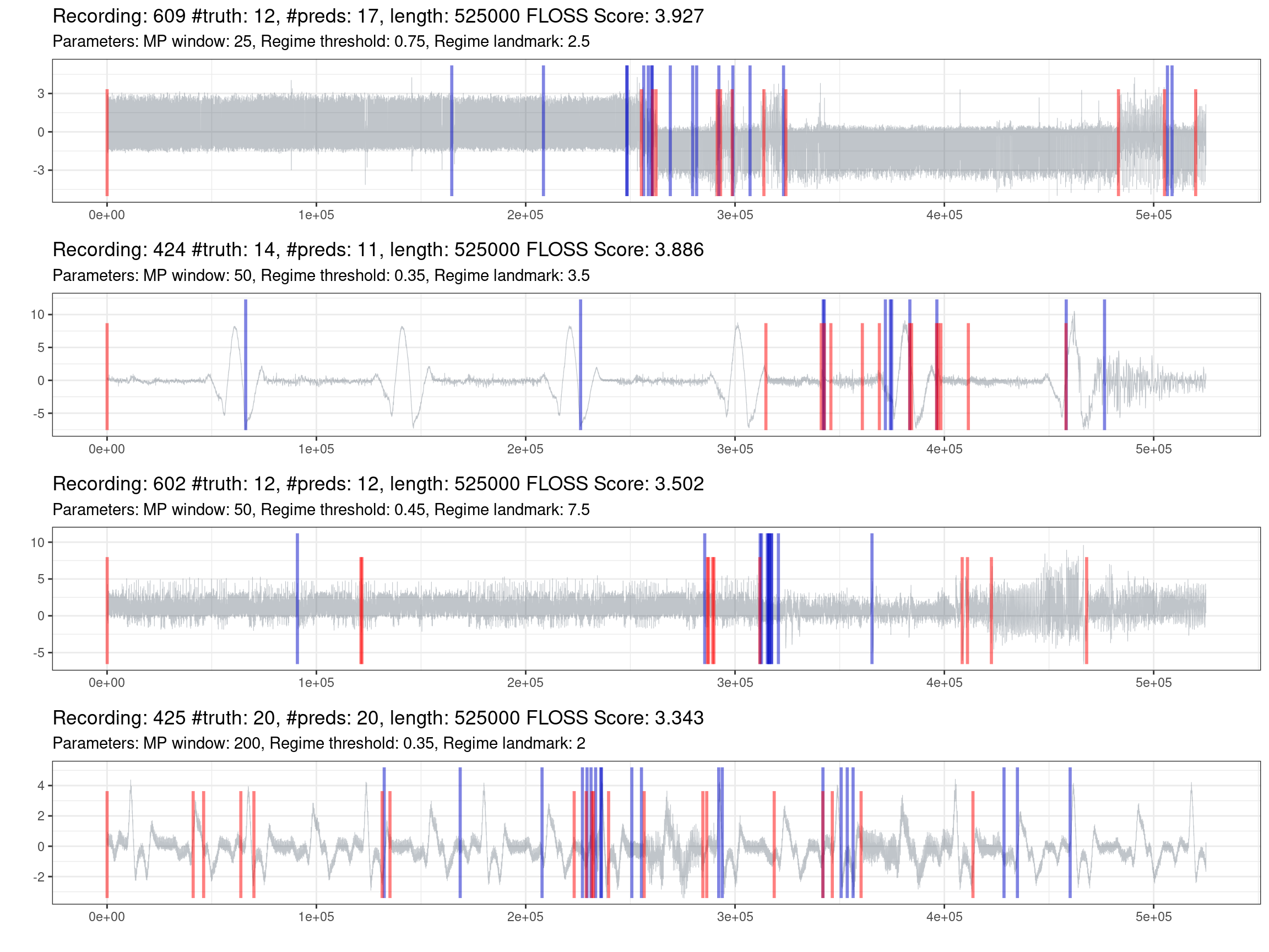
Figure 1.6: Prediction of the worst 30% of recordings (red is the truth, blue are the predictions).
Fig. 1.7 shows the best performances of the best recordings.
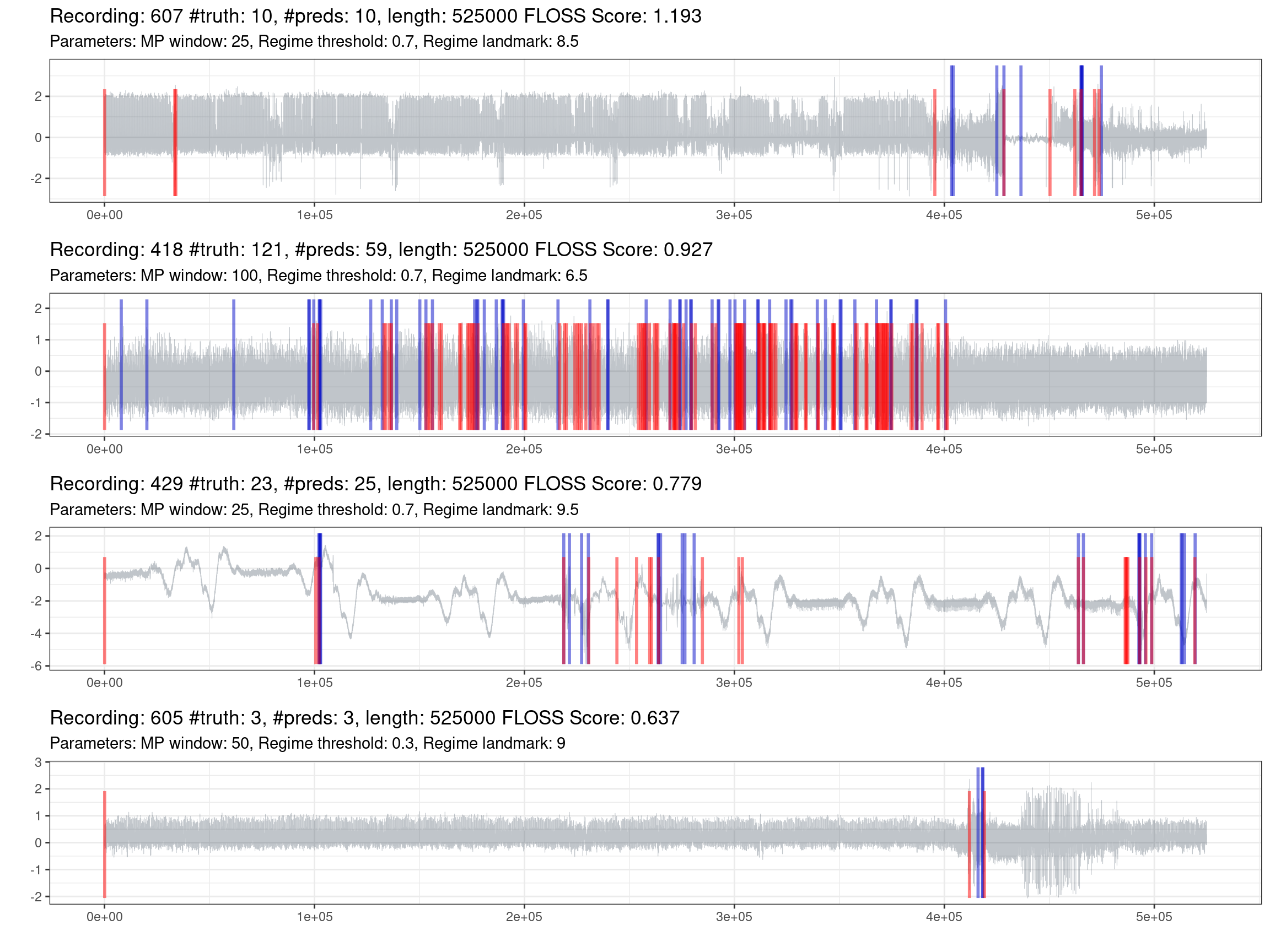
Figure 1.7: Prediction of the best 30% of recordings (red is the truth, blue are the predictions).
An online interactive version of all the datasets and predictions can be accessed at Shiny app.
1.4.2 By model
Fig. 1.8 shows the distribution of the FLOSS score of the 10% worst (left side) and 10% best models across the recordings (right side). The bluish color highlights the models with SD below 3 and IQR below 1.
Here again, we can compare with the previous article and see an improvement in the performance, as the models present lower SD and IQR.

Figure 1.8: Violin plot showing the distribution of the FLOSS score achieved by all tested models during the inner ressample. The left half shows the models with the worst performances (top 10), whereas the right half shows the models with the best performances (top 10). The models are sorted (left-right) by the mean score (top) and by the median (below). Ties are sorted by the SD and IQR, respectively. The bluish colors highlights models with an SD below 10 and IQR below 10.
Fig. 1.9 the performance of the six best models. They are ordered from left to right, from the worst record to the best record. The top model is the one with the lowest mean across the scores. The blue line indicates the mean score, and the red line the median score. The scores above 3 are squished in the plot and colored according to the scale in the legend. Notice the improvement on the blue and red lines compared to the previous article.

Figure 1.9: Performances of the best 6 models across all inner resample of recordings. The recordings are ordered by score, from the worst to the best. Each plot shows one model, starting from the best one. The red line indicates the median score of the model. The blue line indicates the mean score of the model. The gray line limits the zero-score region.
References
─ Session info ───────────────────────────────────────────────────────────────
 setting  value
 version  R version 4.3.1 (2023-06-16)
 os       Ubuntu 22.04.3 LTS
 system   x86_64, linux-gnu
 ui       X11
 language (EN)
 collate  en_US.UTF-8
 ctype    en_US.UTF-8
 tz       Europe/Lisbon
 date     2023-12-10
 pandoc   2.17.0.1 @ /usr/bin/ (via rmarkdown)

─ Packages ───────────────────────────────────────────────────────────────────
 package      * version     date (UTC) lib source
 askpass        1.1         2019-01-13 [1] CRAN (R 4.3.0)
 backports      1.4.1       2021-12-13 [1] CRAN (R 4.3.1)
 base64url      1.4         2018-05-14 [1] CRAN (R 4.3.0)
 bit            4.0.5       2022-11-15 [1] CRAN (R 4.3.0)
 bit64          4.0.5       2020-08-30 [1] CRAN (R 4.3.0)
 bookdown       0.35.1      2023-08-13 [1] Github (rstudio/bookdown@661567e)
 bslib          0.5.1       2023-08-11 [1] CRAN (R 4.3.1)
 cachem         1.0.8       2023-05-01 [1] CRAN (R 4.3.0)
 callr          3.7.3       2022-11-02 [1] CRAN (R 4.3.1)
 checkmate      2.2.0       2023-04-27 [1] CRAN (R 4.3.0)
 class          7.3-22      2023-05-03 [2] CRAN (R 4.3.1)
 cli            3.6.1       2023-03-23 [1] CRAN (R 4.3.1)
 codetools      0.2-19      2023-02-01 [2] CRAN (R 4.3.0)
 colorspace     2.1-0       2023-01-23 [1] CRAN (R 4.3.0)
 crayon         1.5.2       2022-09-29 [1] CRAN (R 4.3.1)
 credentials    1.3.2       2021-11-29 [1] CRAN (R 4.3.0)
 data.table     1.14.8      2023-02-17 [1] CRAN (R 4.3.0)
 dbarts         0.9-23      2023-01-23 [1] CRAN (R 4.3.0)
 debugme        1.1.0       2017-10-22 [1] CRAN (R 4.3.0)
 devtools       2.4.5       2022-10-11 [1] CRAN (R 4.3.0)
 dials          1.2.0       2023-04-03 [1] CRAN (R 4.3.0)
 DiceDesign     1.9         2021-02-13 [1] CRAN (R 4.3.0)
 digest         0.6.33      2023-07-07 [1] CRAN (R 4.3.1)
 dplyr          1.1.3       2023-09-03 [1] CRAN (R 4.3.1)
 ellipsis       0.3.2       2021-04-29 [1] CRAN (R 4.3.0)
 evaluate       0.21        2023-05-05 [1] CRAN (R 4.3.0)
 fansi          1.0.4       2023-01-22 [1] CRAN (R 4.3.0)
 farver         2.1.1       2022-07-06 [1] CRAN (R 4.3.0)
 fastmap        1.1.1       2023-02-24 [1] CRAN (R 4.3.0)
 fastshap       0.0.7       2021-12-06 [1] CRAN (R 4.3.0)
 forcats        1.0.0       2023-01-29 [1] CRAN (R 4.3.0)
 foreach        1.5.2       2022-02-02 [1] CRAN (R 4.3.0)
 fs             1.6.3       2023-07-20 [1] CRAN (R 4.3.1)
 furrr          0.3.1       2022-08-15 [1] CRAN (R 4.3.0)
 future         1.33.0      2023-07-01 [1] CRAN (R 4.3.1)
 future.apply   1.11.0      2023-05-21 [1] CRAN (R 4.3.1)
 future.callr   0.8.2       2023-08-09 [1] CRAN (R 4.3.1)
 generics       0.1.3       2022-07-05 [1] CRAN (R 4.3.0)
 gert           1.9.3       2023-08-07 [1] CRAN (R 4.3.1)
 getPass        0.2-2       2017-07-21 [1] CRAN (R 4.3.0)
 ggplot2      * 3.4.3       2023-08-14 [1] CRAN (R 4.3.1)
 git2r          0.32.0.9000 2023-06-30 [1] Github (ropensci/git2r@9c42d41)
 gittargets   * 0.0.6.9000  2023-05-05 [1] Github (wlandau/gittargets@2d448ff)
 globals        0.16.2      2022-11-21 [1] CRAN (R 4.3.0)
 glue         * 1.6.2       2022-02-24 [1] CRAN (R 4.3.1)
 gower          1.0.1       2022-12-22 [1] CRAN (R 4.3.0)
 GPfit          1.0-8       2019-02-08 [1] CRAN (R 4.3.0)
 gridExtra      2.3         2017-09-09 [1] CRAN (R 4.3.0)
 gtable         0.3.3       2023-03-21 [1] CRAN (R 4.3.0)
 hardhat        1.3.0       2023-03-30 [1] CRAN (R 4.3.0)
 here         * 1.0.1       2020-12-13 [1] CRAN (R 4.3.0)
 highr          0.10        2022-12-22 [1] CRAN (R 4.3.1)
 hms            1.1.3       2023-03-21 [1] CRAN (R 4.3.0)
 htmltools      0.5.6       2023-08-10 [1] CRAN (R 4.3.1)
 htmlwidgets    1.6.2       2023-03-17 [1] CRAN (R 4.3.0)
 httpuv         1.6.11      2023-05-11 [1] CRAN (R 4.3.1)
 httr           1.4.6       2023-05-08 [1] CRAN (R 4.3.1)
 igraph         1.5.1       2023-08-10 [1] CRAN (R 4.3.1)
 ipred          0.9-14      2023-03-09 [1] CRAN (R 4.3.0)
 iterators      1.0.14      2022-02-05 [1] CRAN (R 4.3.0)
 jquerylib      0.1.4       2021-04-26 [1] CRAN (R 4.3.0)
 jsonlite       1.8.7       2023-06-29 [1] CRAN (R 4.3.0)
 kableExtra   * 1.3.4       2021-02-20 [1] CRAN (R 4.3.0)
 knitr          1.43        2023-05-25 [1] CRAN (R 4.3.0)
 labeling       0.4.2       2020-10-20 [1] CRAN (R 4.3.0)
 later          1.3.1       2023-05-02 [1] CRAN (R 4.3.1)
 lattice        0.22-5      2023-10-24 [2] CRAN (R 4.3.1)
 lava           1.7.2.1     2023-02-27 [1] CRAN (R 4.3.0)
 lhs            1.1.6       2022-12-17 [1] CRAN (R 4.3.0)
 lifecycle      1.0.3       2022-10-07 [1] CRAN (R 4.3.1)
 listenv        0.9.0       2022-12-16 [1] CRAN (R 4.3.0)
 lubridate      1.9.2       2023-02-10 [1] CRAN (R 4.3.0)
 magrittr       2.0.3       2022-03-30 [1] CRAN (R 4.3.1)
 MASS           7.3-60      2023-05-04 [2] CRAN (R 4.3.1)
 Matrix         1.6-1.1     2023-09-18 [2] CRAN (R 4.3.1)
 memoise        2.0.1       2021-11-26 [1] CRAN (R 4.3.0)
 mgcv           1.9-0       2023-07-11 [2] CRAN (R 4.3.1)
 mime           0.12        2021-09-28 [1] CRAN (R 4.3.0)
 miniUI         0.1.1.1     2018-05-18 [1] CRAN (R 4.3.0)
 modelenv       0.1.1       2023-03-08 [1] CRAN (R 4.3.0)
 munsell        0.5.0       2018-06-12 [1] CRAN (R 4.3.0)
 nlme           3.1-163     2023-08-09 [1] CRAN (R 4.3.1)
 nnet           7.3-19      2023-05-03 [2] CRAN (R 4.3.1)
 openssl        2.1.0       2023-07-15 [1] CRAN (R 4.3.1)
 parallelly     1.36.0      2023-05-26 [1] CRAN (R 4.3.1)
 parsnip        1.1.0       2023-04-12 [1] CRAN (R 4.3.0)
 patchwork    * 1.1.2       2022-08-19 [1] CRAN (R 4.3.0)
 pdp            0.8.1       2023-06-22 [1] Github (bgreenwell/pdp@4f22141)
 pillar         1.9.0       2023-03-22 [1] CRAN (R 4.3.0)
 pkgbuild       1.4.2       2023-06-26 [1] CRAN (R 4.3.1)
 pkgconfig      2.0.3       2019-09-22 [1] CRAN (R 4.3.0)
 pkgload        1.3.2.1     2023-07-08 [1] CRAN (R 4.3.1)
 prettyunits    1.1.1       2020-01-24 [1] CRAN (R 4.3.0)
 processx       3.8.2       2023-06-30 [1] CRAN (R 4.3.1)
 prodlim        2023.03.31  2023-04-02 [1] CRAN (R 4.3.0)
 profvis        0.3.8       2023-05-02 [1] CRAN (R 4.3.1)
 promises       1.2.1       2023-08-10 [1] CRAN (R 4.3.1)
 ps             1.7.5       2023-04-18 [1] CRAN (R 4.3.1)
 purrr          1.0.2       2023-08-10 [1] CRAN (R 4.3.1)
 R6             2.5.1       2021-08-19 [1] CRAN (R 4.3.1)
 Rcpp           1.0.11      2023-07-06 [1] CRAN (R 4.3.1)
 readr          2.1.4       2023-02-10 [1] CRAN (R 4.3.0)
 recipes        1.0.7       2023-08-10 [1] CRAN (R 4.3.1)
 remotes        2.4.2.1     2023-07-18 [1] CRAN (R 4.3.1)
 renv           0.17.3      2023-04-06 [1] CRAN (R 4.3.1)
 rlang          1.1.1       2023-04-28 [1] CRAN (R 4.3.0)
 rmarkdown      2.25.1      2023-10-10 [1] Github (rstudio/rmarkdown@65a352e)
 rpart          4.1.21      2023-10-09 [2] CRAN (R 4.3.1)
 rprojroot      2.0.3       2022-04-02 [1] CRAN (R 4.3.1)
 rsample        1.1.1       2022-12-07 [1] CRAN (R 4.3.0)
 rstudioapi     0.15.0      2023-07-07 [1] CRAN (R 4.3.1)
 rvest          1.0.3       2022-08-19 [1] CRAN (R 4.3.0)
 sass           0.4.7       2023-07-15 [1] CRAN (R 4.3.1)
 scales         1.2.1       2022-08-20 [1] CRAN (R 4.3.0)
 sessioninfo    1.2.2       2021-12-06 [1] CRAN (R 4.3.0)
 shapviz        0.9.1       2023-07-18 [1] CRAN (R 4.3.1)
 shiny          1.7.5       2023-08-12 [1] CRAN (R 4.3.1)
 signal         0.7-7       2021-05-25 [1] CRAN (R 4.3.0)
 stringi        1.7.12      2023-01-11 [1] CRAN (R 4.3.1)
 stringr        1.5.0       2022-12-02 [1] CRAN (R 4.3.1)
 survival       3.5-7       2023-08-14 [2] CRAN (R 4.3.1)
 svglite        2.1.1.9000  2023-05-05 [1] Github (r-lib/svglite@6c1d359)
 sys            3.4.2       2023-05-23 [1] CRAN (R 4.3.1)
 systemfonts    1.0.4       2022-02-11 [1] CRAN (R 4.3.0)
 tarchetypes  * 0.7.7       2023-06-15 [1] CRAN (R 4.3.1)
 targets      * 1.2.2       2023-08-10 [1] CRAN (R 4.3.1)
 tibble       * 3.2.1       2023-03-20 [1] CRAN (R 4.3.0)
 tidyr          1.3.0       2023-01-24 [1] CRAN (R 4.3.0)
 tidyselect     1.2.0       2022-10-10 [1] CRAN (R 4.3.0)
 timechange     0.2.0       2023-01-11 [1] CRAN (R 4.3.0)
 timeDate       4022.108    2023-01-07 [1] CRAN (R 4.3.0)
 timetk         2.8.3       2023-03-30 [1] CRAN (R 4.3.0)
 tune           1.1.1       2023-04-11 [1] CRAN (R 4.3.0)
 tzdb           0.4.0       2023-05-12 [1] CRAN (R 4.3.1)
 urlchecker     1.0.1       2021-11-30 [1] CRAN (R 4.3.0)
 usethis        2.2.2.9000  2023-07-17 [1] Github (r-lib/usethis@467ff57)
 utf8           1.2.3       2023-01-31 [1] CRAN (R 4.3.0)
 uuid           1.1-0       2022-04-19 [1] CRAN (R 4.3.0)
 vctrs          0.6.3       2023-06-14 [1] CRAN (R 4.3.1)
 vip            0.3.2       2020-12-17 [1] CRAN (R 4.3.0)
 viridisLite    0.4.2       2023-05-02 [1] CRAN (R 4.3.1)
 visNetwork   * 2.1.2       2022-09-29 [1] CRAN (R 4.3.0)
 vroom          1.6.3       2023-04-28 [1] CRAN (R 4.3.1)
 webshot        0.5.5       2023-06-26 [1] CRAN (R 4.3.1)
 whisker        0.4.1       2022-12-05 [1] CRAN (R 4.3.0)
 withr          2.5.0       2022-03-03 [1] CRAN (R 4.3.1)
 workflowr    * 1.7.0       2021-12-21 [1] CRAN (R 4.3.0)
 workflows      1.1.3       2023-02-22 [1] CRAN (R 4.3.0)
 xfun           0.40        2023-08-09 [1] CRAN (R 4.3.1)
 xgboost        1.7.5.1     2023-03-30 [1] CRAN (R 4.3.0)
 xml2           1.3.5       2023-07-06 [1] CRAN (R 4.3.1)
 xtable         1.8-4       2019-04-21 [1] CRAN (R 4.3.0)
 xts            0.13.1      2023-04-16 [1] CRAN (R 4.3.0)
 yaml           2.3.7       2023-01-23 [1] CRAN (R 4.3.1)
 yardstick      1.0.0.9000  2023-05-25 [1] Github (tidymodels/yardstick@90ab794)
 zoo            1.8-12      2023-04-13 [1] CRAN (R 4.3.0)

 [1] /workspace/.cache/R/renv/proj_libs/develop-e2b961e1/R-4.3/x86_64-pc-linux-gnu
 [2] /usr/lib/R/library

──────────────────────────────────────────────────────────────────────────────