Regime changes
Francisco Bischoff
on November 30, 2023
Last updated: 2023-11-30
Checks: 7 0
Knit directory:
develop/docs/
This reproducible R Markdown analysis was created with workflowr (version 1.7.0). The Checks tab describes the reproducibility checks that were applied when the results were created. The Past versions tab lists the development history.
Great! Since the R Markdown file has been committed to the Git repository, you know the exact version of the code that produced these results.
Great job! The global environment was empty. Objects defined in the global environment can affect the analysis in your R Markdown file in unknown ways. For reproduciblity it’s best to always run the code in an empty environment.
The command set.seed(20201020) was run prior to running the code in the R Markdown file.
Setting a seed ensures that any results that rely on randomness, e.g.
subsampling or permutations, are reproducible.
Great job! Recording the operating system, R version, and package versions is critical for reproducibility.
Nice! There were no cached chunks for this analysis, so you can be confident that you successfully produced the results during this run.
Great job! Using relative paths to the files within your workflowr project makes it easier to run your code on other machines.
Great! You are using Git for version control. Tracking code development and connecting the code version to the results is critical for reproducibility.
The results in this page were generated with repository version c772fa0. See the Past versions tab to see a history of the changes made to the R Markdown and HTML files.
Note that you need to be careful to ensure that all relevant files for the
analysis have been committed to Git prior to generating the results (you can
use wflow_publish or wflow_git_commit). workflowr only
checks the R Markdown file, but you know if there are other scripts or data
files that it depends on. Below is the status of the Git repository when the
results were generated:
Ignored files:
    Ignored:    .Renviron
    Ignored:    .Rhistory
    Ignored:    .docker/
    Ignored:    .luarc.json
    Ignored:    analysis/figure/
    Ignored:    analysis/shiny/rsconnect/
    Ignored:    analysis/shiny_land/rsconnect/
    Ignored:    analysis/shiny_ventricular/rsconnect/
    Ignored:    analysis/shiny_vtachy/rsconnect/
    Ignored:    dev/
    Ignored:    inst/extdata/
    Ignored:    renv/staging/
    Ignored:    tmp/
Note that any generated files, e.g. HTML, png, CSS, etc., are not included in this status report because it is ok for generated content to have uncommitted changes.
These are the previous versions of the repository in which changes were made
to the R Markdown (analysis/regime_optimize.Rmd) and HTML (docs/regime_optimize.html)
files. If you’ve configured a remote Git repository (see
?wflow_git_remote), click on the hyperlinks in the table below to
view the files as they were in that past version.
| File | Version | Author | Date | Message |
|---|---|---|---|---|
| Rmd | c772fa0 | Francisco Bischoff | 2023-11-30 | update floss |
| Rmd | 5636465 | Francisco Bischoff | 2023-10-05 | regime 2 wip |
| html | 5636465 | Francisco Bischoff | 2023-10-05 | regime 2 wip |
| Rmd | 4887954 | Francisco Bischoff | 2023-08-13 | update report |
| html | 4887954 | Francisco Bischoff | 2023-08-13 | update report |
| Rmd | 7bf2605 | GitHub | 2023-08-13 | Feature/classification (#152) |
| html | f9f551d | Francisco Bischoff | 2022-10-06 | Build site. |
| html | dbbd1d6 | Francisco Bischoff | 2022-08-22 | Squashed commit of the following: |
| html | de21180 | Francisco Bischoff | 2022-08-21 | Squashed commit of the following: |
| html | 5943a09 | Francisco Bischoff | 2022-07-21 | Build site. |
| Rmd | 3328477 | Francisco Bischoff | 2022-07-21 | Build site. |
| html | 3328477 | Francisco Bischoff | 2022-07-21 | Build site. |
| Rmd | 03d1e68 | Francisco Bischoff | 2022-07-19 | Squashed commit of the following: |
| Rmd | 0c54350 | Francisco Bischoff | 2022-06-10 | regimes |
| Rmd | a6f0406 | Francisco Bischoff | 2022-06-08 | optimize |
| Rmd | 441629f | Francisco Bischoff | 2022-05-31 | begining analysis |
1 Regime changes optimization
In this article, we will interchangeably use the words parameter, variable, and feature.
1.1 Current pipeline
Figure 1.1: FLOSS pipeline.
1.2 Tuning process
As we have seen previously, the FLOSS algorithm is built on top of the Matrix Profile (MP). Thus, we have proposed several parameters that may or not impact the FLOSS prediction performance.
The variables for building the MP are:
mp_threshold: the minimum similarity value to be considered for 1-NN.time_constraint: the maximum distance to look for the nearest neighbor.window_size: the default parameter always used to build an MP.
Later, the FLOSS algorithm also has a parameter that needs tuning to optimize the prediction:
regime_threshold: the threshold below which a regime change is considered.
Using the tidymodels framework, we performed a basic grid search on all these parameters, followed by a bayesian search trying to finetune the parameters.
The workflow is as follows:
- From a total of 229 records, a set of 171 records were selected for tuning, and 58 records were held out.
- From these 171 records, a 5-fold cross-validation was performed two times. Here is where the grid search was performed (Figs. 1.2 and 1.3).
- The best ten models from the cross-validation (5 models from each time) were then evaluated on the hold-out set. Table 1.1.
Fig. 1.2 shows the performance achieved individually during the cross-validation for each parameter. The plot shows the default performance metric (floss_error_macro) and another version (floss_error_micro) where the error is computed globally, being less prone to individual record errors.

Figure 1.2: Marginal plot of all parameters searched during the cross-validation. The first line shows the default performance metric (macro), which is the average of the scores of every recording in the resamples. The line below shows another metric (micro) which does not take into account the length of every recording but is later normalized by the total length of the resample. Lower values are better.
Fig. 1.3 shows the performance across all cross-validation folds for every iteration of the bayes search.

Figure 1.3: Parameters exploration using Bayesian optimization. The plots show the performances across all cross-validation folds on every iteration of the bayes search. The first line shows the results of the first repetition, and the second line during the second repetition. The values on the left are shown in the default metric (macro). On the right side, the values are shown in the micro metric. The iteration ‘Zero’ is the initial grid search.
| Version | Author | Date |
|---|---|---|
| 3328477 | Francisco Bischoff | 2022-07-21 |
Table 1.1 shows the performance of the best ten models on the hold-out set (a set of records that was never used for training).
| # | Time Constraint | MP Threshold | Window Size | Regime Threshold | FLOSS Score |
|---|---|---|---|---|---|
| 1 | 1350 | 0.3 | 100 | 0.5 | 0.676 |
| 2 | 1350 | 0.3 | 100 | 0.5 | 0.678 |
| 3 | 1850 | 0.1 | 125 | 0.4 | 0.729 |
| 4 | 1850 | 0.1 | 125 | 0.4 | 0.734 |
| 5 | 1950 | 0.2 | 100 | 0.5 | 0.740 |
| 6 | 1400 | 0.3 | 125 | 0.5 | 0.760 |
1.3 Parameters analysis
The above process was an example of parameter tuning seeking the best model for a given set of parameters. It used a nested cross-validation procedure that aims to find the best combination of parameters and avoid overfitting.
While this process is powerful and robust, it does not show us the importance of each parameter. At least one parameter has been introduced by reasoning about the problem (mp_threshold), but how important it (and other parameters) is for predicting regime changes?
For example, the process above took 4 days, 20 hours, and 15 minutes to complete the grid search using an Intel(R) Xeon(R) Silver 4210R @ 2.40 GHz server. Notice that about 133 different combinations of parameters were tested on computing the MP (not FLOSS, the regime_threshold), 5 folds, 2 times each. That sums up about 35.2 x 10⁹ all-pairs Euclidean distances computed on less than 5 days (on CPU, not GPU). Not bad.
Another side note on the above process, it is not a “release” environment, so we must consider lots of overhead in computation and memory usage that must be taken into account during these five days of grid search. Thus, much time can be saved if we know what parameters are essential for the problem.
In order to check the effect of the parameters on the model, we need to compute the importance of each parameter.
Wei et al. published a comprehensive review on variable importance analysis1.
Our case is not a typical case of variable importance analysis, where a set of features are tested against an outcome. Instead, we have to proxy our analysis by using as outcome the FLOSS performance score and as features (or predictors) the tuning parameters that lead to that score.
That is accomplished by fitting a model using the tuning parameters to predict the FLOSS score and then applying the techniques to compute the importance of each parameter.
For this matter, a Bayesian Additive Regression Trees (BART) model was chosen after an experimental trial with a set of regression models (including glmnet, gbm, mlp) and for its inherent characteristics, which allows being used for model-free variable selection2. The best BART model was selected using 10-fold cross-validation repeated 3 times, having great predictive power with an RMSE around 0.2 and an R2 around 0.99. With this fitted model, we could evaluate each parameter’s importance.
1.3.1 Interactions
Before starting the parameter importance analysis, we need to consider the parameter interactions since this is usually the weak spot of the analysis techniques, as will be discussed later.
The first BART model was fitted using the following parameters:
\[\begin{equation} \begin{aligned} E( score ) &= \alpha + time\_constraint\\ &\quad + mp\_threshold + window\_size\\ &\quad + regime\_threshold \end{aligned} \tag{1.1} \end{equation}\]
After checking the interactions, this is the refitted model:
\[\begin{equation} \begin{aligned} E( score ) &= \alpha + time\_constraint\\ &\quad + mp\_threshold + window\_size\\ &\quad + regime\_threshold + \left(mp\_threshold \times window\_size\right) \end{aligned} \tag{1.2} \end{equation}\]
Fig. 1.4 shows the variable interaction strength between pairs of variables. That allows us to verify if there are any significant interactions between the variables. Using the information from the first model fit, equation (1.1), we see that mp_threshold interacts strongly with window_size. After refitting, taking into account this interaction, we see that the interaction strength graphic is much better, equation (1.2).
![Variable interactions strenght using feature importance ranking measure (FIRM) approach [@Greenwell2018]. A) Shows strong interaction between `mp_threshold` and `window_size`. B) Refitting the model with this interaction taken into account, the strength is substantially reduced.](figure/regime_optimize.Rmd/interaction-1.svg)
Figure 1.4: Variable interactions strenght using feature importance ranking measure (FIRM) approach3. A) Shows strong interaction between mp_threshold and window_size. B) Refitting the model with this interaction taken into account, the strength is substantially reduced.
1.3.2 Importance
After evaluating the interactions, we then can perform the analysis of the variable importance. The goal is to understand how the FLOSS score behaves when we change the parameters.
Here is a brief overview of the different techniques:
1.3.2.1 Feature Importance Ranking Measure (FIRM)
The FIRM is a variance-based method. This implementation uses the ICE curves to quantify each feature effect which is more robust than partial dependance plots (PDP)4.
It is also helpful to inspect the ICE curves to uncover some heterogeneous relationships with the outcome5.
Advantages:
- Has a causal interpretation (for the model, not for the real world)
- ICE curves can uncover heterogeneous relationships
Disadvantages:
- The method does not take into account interactions.
1.3.2.2 Permutation
The Permutation method was introduced by Breiman in 20016 for Random Forest, and the implementation used here is a model-agnostic version introduced by Fisher et al. in 20197. A feature is “unimportant” if shuffling its values leaves the model error unchanged, assuming that the model has ignored the feature for the prediction.
Advantages:
- Easy interpretation: the importance is the increase in model error when the feature’s information is destroyed.
- No interactions: the interaction effects are also destroyed by permuting the feature values.
Disadvantages:
- It is linked to the model error: not a disadvantage per se, but may lead to misinterpretation if the goal is to understand how the output varies, regardless of the model’s performance. For example, if we want to measure the robustness of the model when someone tampers the features, we want to know the model variance explained by the features. Model variance (explained by the features) and feature importance correlate strongly when the model generalizes well (it is not overfitting).
- Correlations: If features are correlated, the permutation feature importance can be biased by unrealistic data instances. Thus we need to be careful if there are strong correlations between features.
1.3.2.3 SHAP
The SHAP feature importance8 is an alternative to permutation feature importance. The difference between both is that Permutation feature importance is based on the decrease in model performance, while SHAP is based on the magnitude of feature attributions.
Advantages:
- It is not linked to the model error: as the underlying concept of SHAP is the Shapley value, the value attributed to each feature is related to its contribution to the output value. If a feature is important, its addition will significantly affect the output.
Disadvantages:
- Computer time: Shapley value is a computationally expensive method and usually is computed using Montecarlo simulations.
- The Shapley value can be misinterpreted: The Shapley value of a feature value is not the difference of the predicted value after removing the feature from the model training. The interpretation of the Shapley value is: “Given the current set of feature values, the contribution of a feature value to the difference between the actual prediction and the mean prediction is the estimated Shapley value”5.
- Correlations: As with other permutation methods, the SHAP feature importance can be biased by unrealistic data instances when features are correlated.
1.3.3 Importance analysis
Using the three techniques above simultaneously allows a broad comparison of the model behavior4. All three methods are model-agnostic (separates interpretation from the model), but as we have seen above, each method has its advantages and disadvantages5.
Fig. 1.5 then shows the variable importance using three methods: Feature Importance Ranking Measure (FIRM) using Individual Conditional Expectation (ICE), Permutation-based, and Shapley Additive explanations (SHAP). The first line of this figure shows that the interaction between mp_threshold and window_size obscures the results, where except for time_constraint, the other variables have similar importance. In the second line, the most important feature that all three methods agree on is the regime_threshold.

Figure 1.5: Variables importances using three different methods. A) Feature Importance Ranking Measure using ICE curves. B) Permutation method. C) SHAP (100 iterations). Line 1 refers to the original fit, and line 2 to the re-fit, taking into account the interactions between variables (Fig. 1.4).
Fig. 1.6 and 1.7 show the effect of each feature on the FLOSS score. The main differences before and after removing the interactions are the magnitude of the less important features and the shape of time_constraint that initially had a valley around 1600. However, it seems that it flats out.

Figure 1.6: This shows the effect each variable has on FLOSS score. This plot doesn’t take into account the variable interactions.

Figure 1.7: This shows the effect each variable has on FLOSS score taking into account the interactions.
We then can see that in this setting, the only variables worthing tuning are the window_size that is a required parameter for the Matrix Profile and seems to give better results with lower window sizes, and the regime_threshold that is a required parameter for FLOSS and seems to have a better performance around 0.4. As time_constraint flats out, this parameter can be, at this moment, removed from the model. mp_threshold also seems not to be a good parameter to keep so that we can leave it at its default of zero.
According to the FLOSS paper9, the window_size is a feature that can be tuned; nevertheless, the results appear to be similar in a reasonably wide range of windows. At this point, we see that the window size of 100 (which is less than half of a second) did not reach a minimum, suggesting that smaller windows could have better performances.
On the other hand, the regime_threshold seems to have an optimal value, but due to a lack of resources until this date, we could not test another variable (that is worth tuning, now that we know that we can have a shorter window size) that is the regime_landmark.
This parameter was fixed to the value of 3 seconds from the last observation (at 250hz, this means the position 750 from the end). It can be shifted, for example, from 1 second to a maximum of 10 seconds (the official limit to fire the alarm) and assess the Corrected Arc Counts in a location with more information about the new regime and is less distorted by the edges.
A preliminary result of the ongoing tuning (with regime_landmark) is depicted below (still a work in progress). It shows us two prediction paths, and assuming (by eye) that the more vertical the line, the less interference will be on the prediction, this means that having settled the window_size and a regime_landmark, the regime_threshold will have the best tuning value for each case.
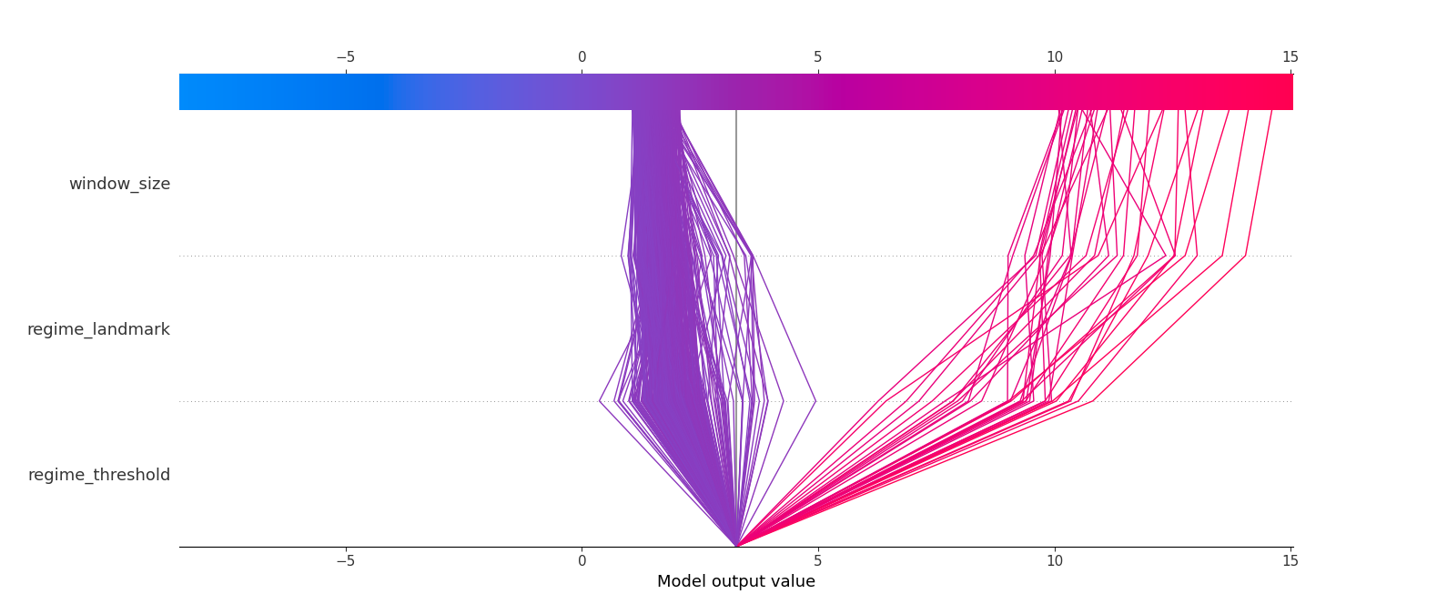
Figure 1.8: Multioutput decision plot.
| Version | Author | Date |
|---|---|---|
| 03d1e68 | Francisco Bischoff | 2022-07-19 |
1.4 Visualizing the predictions
At this point, the grid search tested a total of 233 models with resulting (individual) scores from 0.0009 to 1279.4 (Q25: 0.3498, Q50: 1.0930, Q75: 2.4673).
1.4.1 By recording
First, we will visualize how the models (in general) performed throughout the individual recordings.
Fig. 1.9 shows a violin plot of equal areas clipped to the minimum value. The blue color indicates the recordings with a small IQR (interquartile range) of model scores. We see on the left half 10% of the recordings with the worst minimum score, and on the right half, 10% of the recordings with the best minimum score.
Next, we will visualize some of these predictions to understand why some recordings were difficult to segment. For us to have a simple baseline: a recording with just one regime change, and the model predicts exactly one regime change, but far from the truth, the score will be roughly 1.

Figure 1.9: Violin plot showing the distribution of the FLOSS score achieved by all tested models by recording. The left half shows the recordings that were difficult to predict (10% overall), whereas the right half shows the recordings that at least one model could achieve a good prediction (10% overall). The recordings are sorted (left-right) by the minimum (best) score achieved in descending order, and ties are sorted by the median of all recording scores. The blue color highlights recordings where models had an IQR variability of less than one. As a simple example, a recording with just one regime change, and the model predicts exactly one change, far from the truth, the score will be roughly 1.
Fig. 1.10 shows the best effort in predicting the most complex recordings. One information not declared before is that if the model does not predict any change, it will put a mark on the zero position. On the other side, the truth markers positioned at the beginning and the end of the recording were removed, as these locations lack information and do not represent a streaming setting.
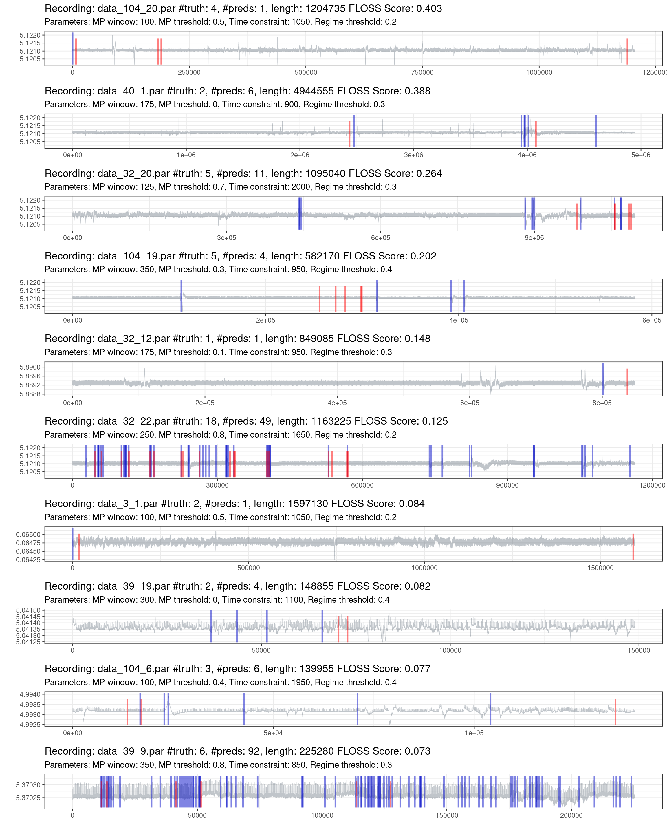
Figure 1.10: Prediction of the worst 10% of recordings (red is the truth, blue are the predictions).
Fig. 1.11 shows the best performances of the best recordings. Notice that there are recordings with a significant duration and few regime changes, making it hard for a “trivial model” to predict randomly.
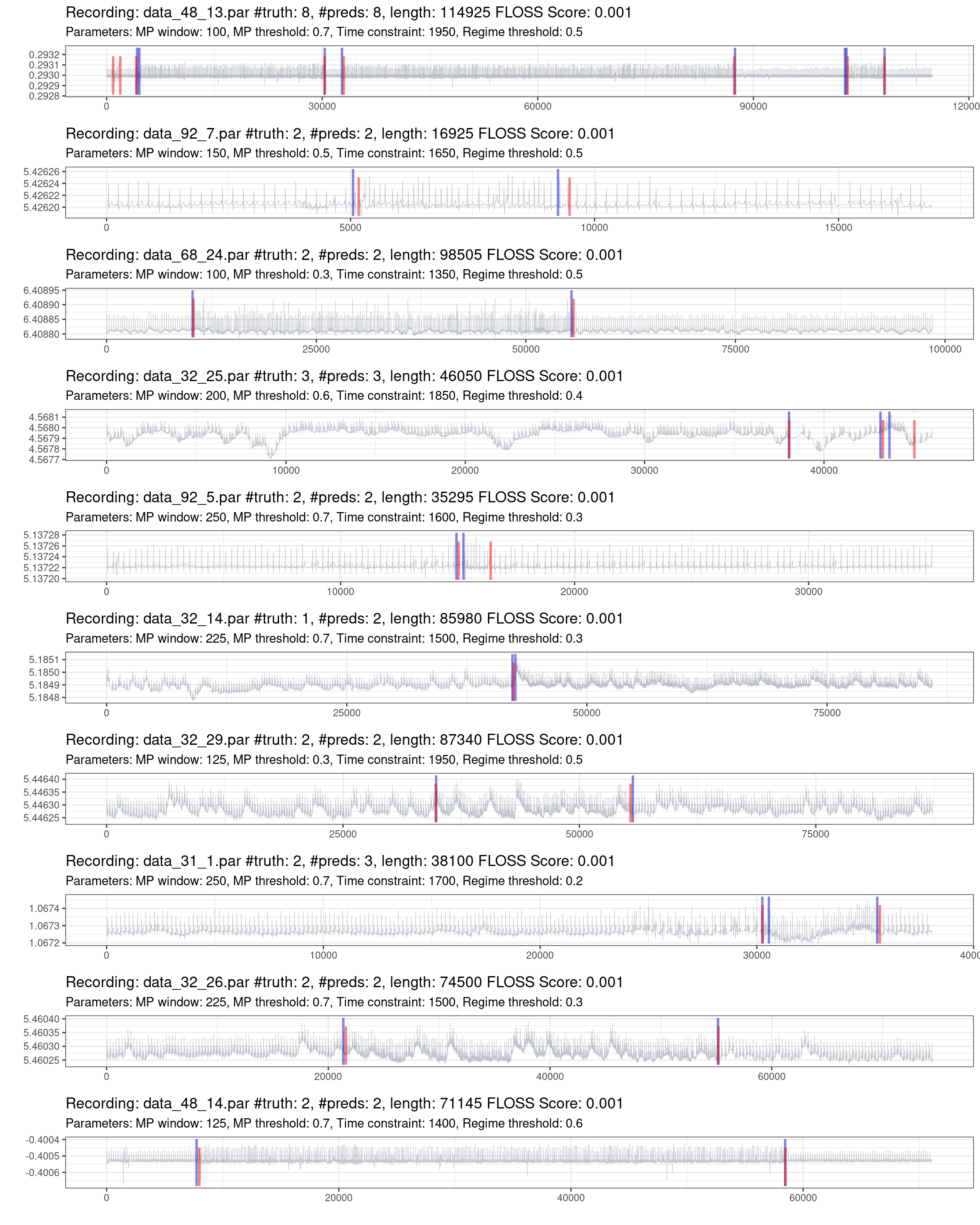
Figure 1.11: Prediction of the best 10% of recordings (red is the truth, blue are the predictions).
An online interactive version of all the datasets and predictions can be accessed at Shiny app.
A work-in-progress version for the finer grid-search over the regime_landmark is available here: Shiny app, which shows promising results.
1.4.2 By model
Fig. 1.12 shows the distribution of the FLOSS score of the 10% worst (left side) and 10% best models across the recordings (right side). The bluish color highlights the models with SD below 1 and IQR below 1.

Figure 1.12: Violin plot showing the distribution of the FLOSS score achieved by all tested models during the inner ressample. The left half shows the models with the worst performances (10% overall), whereas the right half shows the models with the best performances (10% overall). The models are sorted (left-right) by the mean score (top) and by the median (below). Ties are sorted by the SD and IQR, respectively. The bluish colors highlights models with an SD below 1 and IQR below 1.
Fig. 1.13 the performance of the six best models across all inner resamples. They are ordered from left to right, from the worst record to the best record. The top model is the one with the lowest mean across the scores. The blue line indicates the mean score, and the red line the median score. The scores above 3 are squished in the plot and colored according to the scale in the legend.

Figure 1.13: Performances of the best 6 models across all inner resample of recordings. The recordings are ordered by score, from the worst to the best. Each plot shows one model, starting from the best one. The red line indicates the median score of the model. The blue line indicates the mean score of the model. The gray line limits the zero-score region. The plot is limited on the “y” axis, and the scores above this limit are shown in color.
We can see that some records (namely #26, #45, #122, #124, #132, #162) are contained in the set of “difficult” records shown in Fig. 1.9.
2 Current status
That is the current status of the project. The optimization using the regime_landmark feature is in progress, and the following article will discuss all the findings.
In parallel, another score measure is being developed based on the concept of Precision and Recall, but for time-series10. It is expected that such a score measure will help to choose the best final model where most of the significant regime changes are detected, keeping a reasonable amount of false positives that will be ruled out further by the classification algorithm.
References
─ Session info ───────────────────────────────────────────────────────────────
 setting  value
 version  R version 4.3.1 (2023-06-16)
 os       Ubuntu 22.04.3 LTS
 system   x86_64, linux-gnu
 ui       X11
 language (EN)
 collate  en_US.UTF-8
 ctype    en_US.UTF-8
 tz       Europe/Lisbon
 date     2023-11-30
 pandoc   2.17.0.1 @ /usr/bin/ (via rmarkdown)

─ Packages ───────────────────────────────────────────────────────────────────
 package      * version     date (UTC) lib source
 askpass        1.1         2019-01-13 [1] CRAN (R 4.3.0)
 backports      1.4.1       2021-12-13 [1] CRAN (R 4.3.1)
 base64url      1.4         2018-05-14 [1] CRAN (R 4.3.0)
 bit            4.0.5       2022-11-15 [1] CRAN (R 4.3.0)
 bit64          4.0.5       2020-08-30 [1] CRAN (R 4.3.0)
 bookdown       0.35.1      2023-08-13 [1] Github (rstudio/bookdown@661567e)
 bslib          0.5.1       2023-08-11 [1] CRAN (R 4.3.1)
 cachem         1.0.8       2023-05-01 [1] CRAN (R 4.3.0)
 callr          3.7.3       2022-11-02 [1] CRAN (R 4.3.1)
 checkmate      2.2.0       2023-04-27 [1] CRAN (R 4.3.0)
 class          7.3-22      2023-05-03 [2] CRAN (R 4.3.1)
 cli            3.6.1       2023-03-23 [1] CRAN (R 4.3.1)
 codetools      0.2-19      2023-02-01 [2] CRAN (R 4.3.0)
 colorspace     2.1-0       2023-01-23 [1] CRAN (R 4.3.0)
 crayon         1.5.2       2022-09-29 [1] CRAN (R 4.3.1)
 credentials    1.3.2       2021-11-29 [1] CRAN (R 4.3.0)
 data.table     1.14.8      2023-02-17 [1] CRAN (R 4.3.0)
 dbarts         0.9-23      2023-01-23 [1] CRAN (R 4.3.0)
 debugme        1.1.0       2017-10-22 [1] CRAN (R 4.3.0)
 devtools       2.4.5       2022-10-11 [1] CRAN (R 4.3.0)
 dials          1.2.0       2023-04-03 [1] CRAN (R 4.3.0)
 DiceDesign     1.9         2021-02-13 [1] CRAN (R 4.3.0)
 digest         0.6.33      2023-07-07 [1] CRAN (R 4.3.1)
 dplyr          1.1.3       2023-09-03 [1] CRAN (R 4.3.1)
 ellipsis       0.3.2       2021-04-29 [1] CRAN (R 4.3.0)
 evaluate       0.21        2023-05-05 [1] CRAN (R 4.3.0)
 fansi          1.0.4       2023-01-22 [1] CRAN (R 4.3.0)
 farver         2.1.1       2022-07-06 [1] CRAN (R 4.3.0)
 fastmap        1.1.1       2023-02-24 [1] CRAN (R 4.3.0)
 fastshap       0.0.7       2021-12-06 [1] CRAN (R 4.3.0)
 forcats        1.0.0       2023-01-29 [1] CRAN (R 4.3.0)
 foreach        1.5.2       2022-02-02 [1] CRAN (R 4.3.0)
 fs             1.6.3       2023-07-20 [1] CRAN (R 4.3.1)
 furrr          0.3.1       2022-08-15 [1] CRAN (R 4.3.0)
 future         1.33.0      2023-07-01 [1] CRAN (R 4.3.1)
 future.apply   1.11.0      2023-05-21 [1] CRAN (R 4.3.1)
 future.callr   0.8.2       2023-08-09 [1] CRAN (R 4.3.1)
 generics       0.1.3       2022-07-05 [1] CRAN (R 4.3.0)
 gert           1.9.3       2023-08-07 [1] CRAN (R 4.3.1)
 getPass        0.2-2       2017-07-21 [1] CRAN (R 4.3.0)
 ggplot2      * 3.4.3       2023-08-14 [1] CRAN (R 4.3.1)
 git2r          0.32.0.9000 2023-06-30 [1] Github (ropensci/git2r@9c42d41)
 gittargets   * 0.0.6.9000  2023-05-05 [1] Github (wlandau/gittargets@2d448ff)
 globals        0.16.2      2022-11-21 [1] CRAN (R 4.3.0)
 glue         * 1.6.2       2022-02-24 [1] CRAN (R 4.3.1)
 gower          1.0.1       2022-12-22 [1] CRAN (R 4.3.0)
 GPfit          1.0-8       2019-02-08 [1] CRAN (R 4.3.0)
 gridExtra      2.3         2017-09-09 [1] CRAN (R 4.3.0)
 gtable         0.3.3       2023-03-21 [1] CRAN (R 4.3.0)
 hardhat        1.3.0       2023-03-30 [1] CRAN (R 4.3.0)
 here         * 1.0.1       2020-12-13 [1] CRAN (R 4.3.0)
 highr          0.10        2022-12-22 [1] CRAN (R 4.3.1)
 hms            1.1.3       2023-03-21 [1] CRAN (R 4.3.0)
 htmltools      0.5.6       2023-08-10 [1] CRAN (R 4.3.1)
 htmlwidgets    1.6.2       2023-03-17 [1] CRAN (R 4.3.0)
 httpuv         1.6.11      2023-05-11 [1] CRAN (R 4.3.1)
 httr           1.4.6       2023-05-08 [1] CRAN (R 4.3.1)
 igraph         1.5.1       2023-08-10 [1] CRAN (R 4.3.1)
 ipred          0.9-14      2023-03-09 [1] CRAN (R 4.3.0)
 iterators      1.0.14      2022-02-05 [1] CRAN (R 4.3.0)
 jquerylib      0.1.4       2021-04-26 [1] CRAN (R 4.3.0)
 jsonlite       1.8.7       2023-06-29 [1] CRAN (R 4.3.0)
 kableExtra   * 1.3.4       2021-02-20 [1] CRAN (R 4.3.0)
 knitr          1.43        2023-05-25 [1] CRAN (R 4.3.0)
 labeling       0.4.2       2020-10-20 [1] CRAN (R 4.3.0)
 later          1.3.1       2023-05-02 [1] CRAN (R 4.3.1)
 lattice        0.22-5      2023-10-24 [2] CRAN (R 4.3.1)
 lava           1.7.2.1     2023-02-27 [1] CRAN (R 4.3.0)
 lhs            1.1.6       2022-12-17 [1] CRAN (R 4.3.0)
 lifecycle      1.0.3       2022-10-07 [1] CRAN (R 4.3.1)
 listenv        0.9.0       2022-12-16 [1] CRAN (R 4.3.0)
 lubridate      1.9.2       2023-02-10 [1] CRAN (R 4.3.0)
 magrittr       2.0.3       2022-03-30 [1] CRAN (R 4.3.1)
 MASS           7.3-60      2023-05-04 [2] CRAN (R 4.3.1)
 Matrix         1.6-1.1     2023-09-18 [2] CRAN (R 4.3.1)
 memoise        2.0.1       2021-11-26 [1] CRAN (R 4.3.0)
 mgcv           1.9-0       2023-07-11 [2] CRAN (R 4.3.1)
 mime           0.12        2021-09-28 [1] CRAN (R 4.3.0)
 miniUI         0.1.1.1     2018-05-18 [1] CRAN (R 4.3.0)
 modelenv       0.1.1       2023-03-08 [1] CRAN (R 4.3.0)
 munsell        0.5.0       2018-06-12 [1] CRAN (R 4.3.0)
 nlme           3.1-163     2023-08-09 [1] CRAN (R 4.3.1)
 nnet           7.3-19      2023-05-03 [2] CRAN (R 4.3.1)
 openssl        2.1.0       2023-07-15 [1] CRAN (R 4.3.1)
 parallelly     1.36.0      2023-05-26 [1] CRAN (R 4.3.1)
 parsnip        1.1.0       2023-04-12 [1] CRAN (R 4.3.0)
 patchwork    * 1.1.2       2022-08-19 [1] CRAN (R 4.3.0)
 pdp            0.8.1       2023-06-22 [1] Github (bgreenwell/pdp@4f22141)
 pillar         1.9.0       2023-03-22 [1] CRAN (R 4.3.0)
 pkgbuild       1.4.2       2023-06-26 [1] CRAN (R 4.3.1)
 pkgconfig      2.0.3       2019-09-22 [1] CRAN (R 4.3.0)
 pkgload        1.3.2.1     2023-07-08 [1] CRAN (R 4.3.1)
 prettyunits    1.1.1       2020-01-24 [1] CRAN (R 4.3.0)
 processx       3.8.2       2023-06-30 [1] CRAN (R 4.3.1)
 prodlim        2023.03.31  2023-04-02 [1] CRAN (R 4.3.0)
 profvis        0.3.8       2023-05-02 [1] CRAN (R 4.3.1)
 promises       1.2.1       2023-08-10 [1] CRAN (R 4.3.1)
 ps             1.7.5       2023-04-18 [1] CRAN (R 4.3.1)
 purrr          1.0.2       2023-08-10 [1] CRAN (R 4.3.1)
 R6             2.5.1       2021-08-19 [1] CRAN (R 4.3.1)
 Rcpp           1.0.11      2023-07-06 [1] CRAN (R 4.3.1)
 readr          2.1.4       2023-02-10 [1] CRAN (R 4.3.0)
 recipes        1.0.7       2023-08-10 [1] CRAN (R 4.3.1)
 remotes        2.4.2.1     2023-07-18 [1] CRAN (R 4.3.1)
 renv           0.17.3      2023-04-06 [1] CRAN (R 4.3.1)
 rlang          1.1.1       2023-04-28 [1] CRAN (R 4.3.0)
 rmarkdown      2.25.1      2023-10-10 [1] Github (rstudio/rmarkdown@65a352e)
 rpart          4.1.21      2023-10-09 [2] CRAN (R 4.3.1)
 rprojroot      2.0.3       2022-04-02 [1] CRAN (R 4.3.1)
 rsample        1.1.1       2022-12-07 [1] CRAN (R 4.3.0)
 rstudioapi     0.15.0      2023-07-07 [1] CRAN (R 4.3.1)
 rvest          1.0.3       2022-08-19 [1] CRAN (R 4.3.0)
 sass           0.4.7       2023-07-15 [1] CRAN (R 4.3.1)
 scales         1.2.1       2022-08-20 [1] CRAN (R 4.3.0)
 sessioninfo    1.2.2       2021-12-06 [1] CRAN (R 4.3.0)
 shiny          1.7.5       2023-08-12 [1] CRAN (R 4.3.1)
 signal         0.7-7       2021-05-25 [1] CRAN (R 4.3.0)
 stringi        1.7.12      2023-01-11 [1] CRAN (R 4.3.1)
 stringr        1.5.0       2022-12-02 [1] CRAN (R 4.3.1)
 survival       3.5-7       2023-08-14 [2] CRAN (R 4.3.1)
 svglite        2.1.1.9000  2023-05-05 [1] Github (r-lib/svglite@6c1d359)
 sys            3.4.2       2023-05-23 [1] CRAN (R 4.3.1)
 systemfonts    1.0.4       2022-02-11 [1] CRAN (R 4.3.0)
 tarchetypes  * 0.7.7       2023-06-15 [1] CRAN (R 4.3.1)
 targets      * 1.2.2       2023-08-10 [1] CRAN (R 4.3.1)
 tibble       * 3.2.1       2023-03-20 [1] CRAN (R 4.3.0)
 tidyr          1.3.0       2023-01-24 [1] CRAN (R 4.3.0)
 tidyselect     1.2.0       2022-10-10 [1] CRAN (R 4.3.0)
 timechange     0.2.0       2023-01-11 [1] CRAN (R 4.3.0)
 timeDate       4022.108    2023-01-07 [1] CRAN (R 4.3.0)
 timetk         2.8.3       2023-03-30 [1] CRAN (R 4.3.0)
 tune           1.1.1       2023-04-11 [1] CRAN (R 4.3.0)
 tzdb           0.4.0       2023-05-12 [1] CRAN (R 4.3.1)
 urlchecker     1.0.1       2021-11-30 [1] CRAN (R 4.3.0)
 usethis        2.2.2.9000  2023-07-17 [1] Github (r-lib/usethis@467ff57)
 utf8           1.2.3       2023-01-31 [1] CRAN (R 4.3.0)
 uuid           1.1-0       2022-04-19 [1] CRAN (R 4.3.0)
 vctrs          0.6.3       2023-06-14 [1] CRAN (R 4.3.1)
 vip            0.3.2       2020-12-17 [1] CRAN (R 4.3.0)
 viridisLite    0.4.2       2023-05-02 [1] CRAN (R 4.3.1)
 visNetwork   * 2.1.2       2022-09-29 [1] CRAN (R 4.3.0)
 vroom          1.6.3       2023-04-28 [1] CRAN (R 4.3.1)
 webshot        0.5.5       2023-06-26 [1] CRAN (R 4.3.1)
 whisker        0.4.1       2022-12-05 [1] CRAN (R 4.3.0)
 withr          2.5.0       2022-03-03 [1] CRAN (R 4.3.1)
 workflowr    * 1.7.0       2021-12-21 [1] CRAN (R 4.3.0)
 workflows      1.1.3       2023-02-22 [1] CRAN (R 4.3.0)
 xfun           0.40        2023-08-09 [1] CRAN (R 4.3.1)
 xml2           1.3.5       2023-07-06 [1] CRAN (R 4.3.1)
 xtable         1.8-4       2019-04-21 [1] CRAN (R 4.3.0)
 xts            0.13.1      2023-04-16 [1] CRAN (R 4.3.0)
 yaml           2.3.7       2023-01-23 [1] CRAN (R 4.3.1)
 yardstick      1.0.0.9000  2023-05-25 [1] Github (tidymodels/yardstick@90ab794)
 zoo            1.8-12      2023-04-13 [1] CRAN (R 4.3.0)

 [1] /workspace/.cache/R/renv/proj_libs/develop-e2b961e1/R-4.3/x86_64-pc-linux-gnu
 [2] /usr/lib/R/library

──────────────────────────────────────────────────────────────────────────────